Why a 1.7% change in the data can move the solution of a linear system by 25%. Derive the condition number as the worst error amplification, compute it from the singular values, prove that forming A-transpose A squares it, and see why the determinant says nothing about it.
M03.8.2L2 Intermediate25 minIn review (what this means)
The maths and code on this page are checked by automated tests on every change, but an independent reader has not signed it off yet. Spot a mistake or a confusing step? Tell us.
Derive the bound that a relative change in b changes the solution of Ax = b by at most kappa(A) times as much.
Compute kappa(A) = sigma_1 / sigma_n by hand for a 2 by 2 matrix and with numpy.linalg.cond.
Prove that kappa(A-transpose A) = kappa(A) squared, and explain what it means for the normal equations.
Explain why the determinant does not measure sensitivity, while the condition number does.
The question
The system with matrix \(\mat{K}\), rows \({(2, 3)}\) and \({(1, 2)}\), and right side \({\vect{b} = (5, 3)}\) has the solution \({\vect{x} = (1, 1)}\). Change the 3 to 3.1, a change of 1.7% in the length of \(\vect{b}\), and the solution jumps to \({(0.7, 1.2)}\), a change of 25%. Data is never exact. Can we tell, before solving, how far a small error in the data can push the answer?
From the last lesson
1. How do the singular values give the 2-norm of a matrix, and what is the smallest stretch?
Show answer
\({\norm{\mat{A}}_2 = \sigma_1}\), the largest stretch; the smallest stretch of a matrix with \(n\) columns is \(\sigma_n\).
2. What inequality does the induced norm give for every vector \(\vect{x}\)?
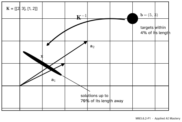
Solving \({\mat{K}\vect{x} = \vect{b}}\) runs the map backwards: from a target \(\vect{b}\) to the input that lands on it. Draw a small disc of possible targets round \(\vect{b}\), all the values the data could have had, and send each back through \({\mat{K}^{-1}}\).
M03.8.2-F1
A disc of targets round \({\vect{b} = (5, 3)}\), each within 4% of \({\norm{\vect{b}}}\), is sent back by \({\mat{K}^{-1}}\) to a long ellipse of solutions round \({\vect{x} = (1, 1)}\). The worst of them is 70% of \({\norm{\vect{x}}}\) away.
The disc does not come back as a disc. The columns of \(\mat{K}\) point almost the same way, so \(\mat{K}\) crushes one direction of the plane nearly flat. Undoing \(\mat{K}\) must blow that direction up again, and a target error that happens to lie along it is blown up with it. The condition number is the worst ratio between the relative size of the solution’s error and the relative size of the data’s error. For \(\mat{K}\) it is about 17.9.
Build it up
Step 1. Errors travel through the inverse. If \({\mat{K}\vect{x} = \vect{b}}\) and \({\mat{K}(\vect{x} + \delta\vect{x})} = {\vect{b} + \delta\vect{b}}\), subtracting gives \({\mat{K}\,\delta\vect{x} = \delta\vect{b}}\), so \({\delta\vect{x} = \mat{K}^{-1}\delta\vect{b}}\).
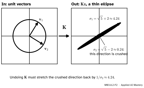
Step 2. How much can the inverse stretch? The unit circle under \(\mat{K}\) becomes an ellipse with semi-axes \({\sigma_1 \approx 4.24}\) and \({\sigma_2 \approx 0.24}\). The inverse sends that ellipse back to the circle, so it stretches the short axis by \({1/\sigma_2 \approx 4.24}\). That is its largest stretch: \({\norm{\mat{K}^{-1}}_2 = 1/\sigma_2}\).
M03.8.2-F2
\(\mat{K}\) maps the unit circle to an ellipse 4.24 long and 0.24 wide. Undoing it multiplies anything along the short axis by \(1/\sigma_2\).
Step 3. How small can the solution be? From \({\vect{b} = \mat{K}\vect{x}}\), \({\norm{\vect{b}} \le \sigma_1\norm{\vect{x}}}\), so \({\norm{\vect{x}} \ge \norm{\vect{b}}/\sigma_1}\). A long target can come from a short input.
Step 4. Divide. The relative error of the solution is at most
In the 2-norm, \({\kappa(\mat{A}) = \sigma_1 / \sigma_n}\).
Proof. From \({\mat{A}\,\delta\vect{x} = \delta\vect{b}}\) we get \({\norm{\delta\vect{x}}} = {\norm{\mat{A}^{-1}\delta\vect{b}}} \le {\norm{\mat{A}^{-1}}\,\norm{\delta\vect{b}}}\). From \({\vect{b} = \mat{A}\vect{x}}\) we get \({\norm{\vect{b}}} \le {\norm{\mat{A}}\,\norm{\vect{x}}}\), that is \({1/\norm{\vect{x}}} \le {\norm{\mat{A}}/\norm{\vect{b}}}\). Multiply the two inequalities, whose sides are all positive.
For the 2-norm, write \({\mat{A} = \mat{U}\mat{\Sigma}\mat{V}\T}\). Then \({\mat{A}^{-1} = \mat{V}\mat{\Sigma}^{-1}\mat{U}\T}\), which is again an SVD, with singular values \(1/\sigma_i\). The largest of these is \(1/\sigma_n\), so \({\norm{\mat{A}^{-1}}_2 = 1/\sigma_n}\) and \({\kappa(\mat{A}) = \sigma_1/\sigma_n}\).
The bound is reached. Choose \(\vect{x}\) along \(\vect{v}_1\), so that \({\norm{\vect{b}} = \sigma_1\norm{\vect{x}}}\), and \(\delta\vect{b}\) along \(\vect{u}_n\), so that \({\norm{\delta\vect{x}}} = {\norm{\delta\vect{b}}/\sigma_n}\). Both inequalities in the proof become equalities. No smaller number would do.
\({\kappa(c\,\mat{A}) = \kappa(\mat{A})}\) for any number \(c \ne 0\): the factors \({\abs{c}}\) and \({1/\abs{c}}\) cancel. The determinant, by contrast, is multiplied by \(c^n\).
\({\kappa(\mat{Q}) = 1}\) for an orthogonal matrix, whose singular values are all 1 (M02.10.2).
Errors in the matrix. If instead the matrix is off, \({(\mat{A} + \delta\mat{A})(\vect{x} + \delta\vect{x})} = {\vect{b}}\), subtract \({\mat{A}\vect{x} = \vect{b}}\):
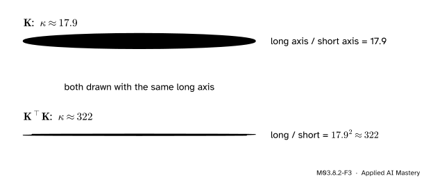
This is the reason, promised in M03.7.2, why the normal equations lose about twice as many digits as QR: they solve a system with matrix \(\mat{A}\T\mat{A}\), whose condition number is squared.
M03.8.2-F3
The unit circle’s image under \(\mat{K}\) and under \(\mat{K}\T\mat{K}\), scaled to the same length. The second is 322 times longer than wide: forming \(\mat{K}\T\mat{K}\) squares the condition number.
Worked example
Find \({\kappa(\mat{K})}\) by hand, and test it with a perturbation.
The relative changes are \({\norm{\delta\vect{b}}/\norm{\vect{b}} = \sqrt{0.0356}/\sqrt{34} \approx 0.0324}\) and \({\norm{\delta\vect{x}}/\norm{\vect{x}} = \sqrt{0.6388}/\sqrt{2} \approx 0.565}\). Their ratio is about 17.5, just under the bound 17.94.
M03.8.2-F4
The condition number of \(\mat{K}\) from its singular values, then a perturbation that comes within 3% of the bound.
The test came close because \({\vect{b} = (5, 3)}\) points almost along \(\vect{u}_1\) and \(\delta\vect{b}\) almost along \(\vect{u}_2\). The code below uses the exact singular vectors and reaches 17.94.
Go deeper: why the golden ratio is hiding in K
Swap the columns of \(\mat{K}\) and you get \(\begin{bmatrix} 3 & 2 \\ 2 & 1 \end{bmatrix} = \mat{F}^3\), the cube of the Fibonacci matrix of M03.2.3. Swapping columns is multiplying by an orthogonal matrix, which changes no singular value. \(\mat{F}^3\) is symmetric with eigenvalues \(\varphi^3\) and \({-\varphi^{-3}}\), so its singular values are \({\varphi^3 = 2 + \sqrt5}\) and \({\varphi^{-3} = \sqrt5 - 2}\), and \({\kappa(\mat{K}) = \varphi^6}\). The worst pair is \(\vect{x}\) along \({(1, \varphi)}\), which \(\mat{K}\) sends to \({\varphi^3(\varphi, 1)}\), and \(\delta\vect{b}\) along \({(1, -\varphi)}\), which \({\mat{K}^{-1}}\) sends to \({\varphi^3(\varphi, -1)}\).
Code
The condition number from the singular values, then checked by experiment.
import numpy as npK = np.array([[2.0, 3.0], [1.0, 2.0]])b, x = np.array([5.0, 3.0]), np.array([1.0, 1.0])U, s, Vh = np.linalg.svd(K)kappa = s[0] / s[-1]print("singular values:", s.round(4), " kappa:", round(kappa, 4), " 9 + 4 sqrt 5 =", round(9+4* np.sqrt(5), 4))def amplification(K, x, db):"""Relative change of the solution divided by relative change of the target.""" b = K @ x dx = np.linalg.solve(K, db)return (np.linalg.norm(dx) / np.linalg.norm(x)) / (np.linalg.norm(db) / np.linalg.norm(b))print("hand test:", round(amplification(K, x, np.array([-0.1, 0.16])), 3))# Ten thousand random perturbations never beat kappa ...rng = np.random.default_rng(0)tries = np.array([amplification(K, x, rng.normal(size=2)) for _ inrange(10_000)])worst = tries.max()print("random tries: median", round(np.median(tries), 2), " worst", round(worst, 3))# ... and the singular vectors reach it exactly.exact = amplification(K, Vh[0], U[:, 1])print("x along v1, db along u2:", round(exact, 4))
singular values: [4.2361 0.2361]  kappa: 17.9443  9 + 4 sqrt 5 = 17.9443
hand test: 17.466
random tries: median 12.51  worst 17.466
x along v1, db along u2: 17.9443
The library call is np.linalg.cond. With no second argument it uses the 2-norm, computed from the SVD; other norms give other numbers of the same size.
In the 1-norm, \({\norm{\mat{K}}_1 = 5}\) and \({\norm{\mat{K}^{-1}}_1 = 5}\), so \({\kappa_1 = 25}\). The exact value depends on the ruler; its size does not.
Explore
M03.8-X1
Condition explorer
Drag the tips of the two columns, or use the sliders, and watch the disc of targets round \(\vect{b}\) come back as an ellipse of solutions round \(\vect{x}\). Line the columns up and the ellipse grows; press Worst x to point \(\vect{x}\) along \(\vect{v}_1\) and see the amplification reach \(\kappa\). Try 0.1 I: a tiny determinant, and a perfectly round result.
Pitfalls
M03.8.2-F5
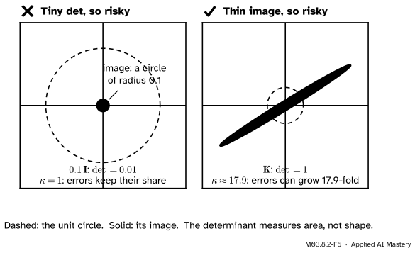
Wrong beside right. \({0.1\,\mat{I}}\) has determinant 0.01 and is perfectly conditioned; \(\mat{K}\) has determinant 1 and amplifies errors almost 18-fold.
“A small determinant means the matrix is nearly singular.”
The determinant measures area, and area mixes size with shape. Scaling a matrix by \(c\) multiplies its \(n\) by \(n\) determinant by \(c^n\) and leaves \(\kappa\) alone. Moler’s example is the 100 by 100 matrix \({0.1\,\mat{I}}\): determinant \({10^{-100}}\), condition number 1. Sensitivity is a question of shape, how thin the image ellipse is, and that is what \(\sigma_1/\sigma_n\) measures. This is the answer promised in M02.8.4.
“A small residual means an accurate answer.”
Suppose a solver returns \({\tilde{\vect{x}} = (1.3, 0.8)}\) for \({\mat{K}\vect{x} = (5, 3)}\). Then \({\mat{K}\tilde{\vect{x}} = (5, 2.9)}\), so the residual \({\vect{b} - \mat{K}\tilde{\vect{x}} = (0, 0.1)}\) is 1.7% of \({\norm{\vect{b}}}\). Yet the error is \({(0.3, -0.2)}\), 25% of \({\norm{\vect{x}}}\). A small residual guarantees a small error only when \(\kappa\) is small (exercise 3).
“Every error is amplified by \(\kappa\).”
The condition number is the worst case. An error amplified that much has to point along the crushed direction, and the target has to point along the stretched one. In the code, half of ten thousand random errors were amplified less than about 12.5 times, and the worst stopped at 17.47, because \({\vect{x} = (1, 1)}\) is not quite along \(\vect{v}_1\). The bound is a guarantee, not a forecast.
Check yourself
Recall
1. Define the condition number, and give its formula in the 2-norm.
Show answer
\({\kappa(\mat{A})} = {\norm{\mat{A}}\,\norm{\mat{A}^{-1}}}\); in the 2-norm, \({\kappa = \sigma_1/\sigma_n}\).
2. State the bound that the condition number gives for \({\mat{A}\vect{x} = \vect{b}}\).
3. Why is \({\kappa(\mat{A}) \ge 1}\) for every invertible matrix?
Show answer
Because \({1} = {\norm{\mat{I}}} = {\norm{\mat{A}\mat{A}^{-1}}} \le {\norm{\mat{A}}\,\norm{\mat{A}^{-1}}}\).
4. What is \({\kappa(\mat{A}\T\mat{A})}\) in terms of \({\kappa(\mat{A})}\), and why does it matter?
Show answer
\({\kappa(\mat{A})^2}\). The normal equations solve a system with \(\mat{A}\T\mat{A}\), so they can lose about twice as many digits as a method that works with \(\mat{A}\) itself, such as QR.
5. What happens to the determinant and to \(\kappa\) when an \(n\) by \(n\) matrix is multiplied by \(c\)?
Show answer
The determinant is multiplied by \(c^n\); the condition number does not change.
Exercises
1.★ Find \(\kappa_2\) and the determinant of \({\mat{D} = \operatorname{diag}(4,\ 0.5)}\) and of \(3\mat{D}\). Which is easier to solve accurately?
Show solution
A diagonal matrix with positive entries has those entries as its singular values. So \({\kappa(\mat{D}) = 4/0.5 = 8}\) and \({\det\mat{D} = 2}\). For \({3\mat{D} = \operatorname{diag}(12,\ 1.5)}\), \({\kappa = 12/1.5 = 8}\) again and \({\det = 18}\). Both are equally easy: the factor 3 changes the determinant ninefold and the sensitivity not at all.
2.★★ Show that multiplying by an orthogonal matrix does not change the 2-norm condition number: \({\kappa(\mat{Q}\mat{A}) = \kappa(\mat{A})}\).
Show solution
If \({\mat{A} = \mat{U}\mat{\Sigma}\mat{V}\T}\), then \({\mat{Q}\mat{A}} = {(\mat{Q}\mat{U})\mat{\Sigma}\mat{V}\T}\), and \(\mat{Q}\mat{U}\) has orthonormal columns because \({(\mat{Q}\mat{U})\T(\mat{Q}\mat{U})} = {\mat{U}\T\mat{Q}\T\mat{Q}\mat{U}} = {\mat{I}}\). So this is an SVD of \(\mat{Q}\mat{A}\) with the same \(\mat{\Sigma}\), and \(\sigma_1/\sigma_n\) is unchanged. This is why QR is safe: the step that multiplies by \(\mat{Q}\T\) cannot make a problem worse.
3.★★★ A solver returns \(\tilde{\vect{x}}\) with residual \({\vect{r} = \vect{b} - \mat{A}\tilde{\vect{x}}}\). Prove that \({\norm{\tilde{\vect{x}} - \vect{x}}/\norm{\vect{x}}} \le {\kappa(\mat{A})\,\norm{\vect{r}}/\norm{\vect{b}}}\), and check it on the pitfall’s numbers.
Show solution
Since \({\mat{A}\vect{x} = \vect{b}}\), we have \({\mat{A}(\vect{x} - \tilde{\vect{x}})} = {\vect{b} - \mat{A}\tilde{\vect{x}}} = {\vect{r}}\). So \({\vect{x} - \tilde{\vect{x}}}\) plays the part of \(\delta\vect{x}\) and \(\vect{r}\) the part of \(\delta\vect{b}\) in the theorem, and the bound follows from the same two lines. For \({\tilde{\vect{x}} = (1.3, 0.8)}\): the relative residual is \({0.1/\sqrt{34} \approx 0.0171}\), so the bound allows a relative error up to \({17.94 \times 0.0171 \approx 0.31}\). The actual error is \({\sqrt{0.13}/\sqrt2 \approx 0.255}\), inside the bound.
Summary card
The condition number is the worst factor by which a solve can magnify a relative error.
M03.8.2-F1
A small disc of data, a long ellipse of answers.
\({\kappa(\mat{A})} = {\norm{\mat{A}}\,\norm{\mat{A}^{-1}}} = {\sigma_1/\sigma_n}\) in the 2-norm.
\({\norm{\delta\vect{x}}/\norm{\vect{x}}} \le {\kappa\,\norm{\delta\vect{b}}/\norm{\vect{b}}}\), with equality for \(\vect{x} \parallel \vect{v}_1\), \(\delta\vect{b} \parallel \vect{u}_n\).
Sources. Each was opened and checked against this lesson on 15 November 2026.
Cleve Moler, Numerical Computing with MATLAB, chapter 2, Linear equations, section 2.9, Norms and condition numbers: the condition number as the largest over the smallest stretch, the bound for a change in \(\vect{b}\), \({\kappa \ge 1}\), \({\kappa(c\mat{A}) = \kappa(\mat{A})}\), the 100 by 100 example \({0.1\,\mat{I}}\) with determinant \({10^{-100}}\) and \({\kappa = 1}\), and \({\kappa = \norm{\mat{A}}\,\norm{\mat{A}^{-1}}}\).
NumPy reference, numpy.linalg.cond: the default p=None is the 2-norm computed with the SVD; 1, inf, 'fro' and others are available.
Nicholas Higham, What is a condition number? (2020): \({\kappa(\mat{A})} = {\norm{\mat{A}}\,\norm{\mat{A}^{-1}}}\) as the condition number both of inversion and of the linear system \({\mat{A}\vect{x} = \vect{b}}\).
Ian Goodfellow, Yoshua Bengio and Aaron Courville, Deep Learning, section 4.2, Poor conditioning: the condition number (4.2) and the remark that the sensitivity belongs to the matrix itself, not to rounding during inversion. Its formula uses eigenvalues, which agrees with \(\sigma_1/\sigma_n\) for symmetric matrices.
Next.M03.8.3 Ill-conditioning in data finds large condition numbers in real design matrices, counts the digits they cost, and tries three remedies.