When two features are copies of each other, least squares has infinitely many solutions. The pseudoinverse, built from the SVD, picks the shortest one. Prove why, check the four Penrose conditions, and meet numpy.linalg.pinv and its cut-off.
M03.7.3L2 Intermediate25 minIn review (what this means)
The maths and code on this page are checked by automated tests on every change, but an independent reader has not signed it off yet. Spot a mistake or a confusing step? Tell us.
Describe every least-squares solution of a problem with dependent columns as one solution plus the null space.
Build the pseudoinverse A+ = V Sigma+ U-transpose and prove that A+ b is the shortest least-squares solution.
Find the minimum-norm weights by hand for a design with a duplicated feature, and explain why they do not measure importance.
Check the four Penrose conditions and use numpy.linalg.pinv with its rcond cut-off.
The question
The four points \(x = (1, 2, 3, 4)\), \(y = (2, 3, 5, 6)\) of ML01 have the best line \(y = 1.4x + 0.5\). Now a data pipeline adds a second feature that is just \(2x\): the same quantity in other units, as happens all the time with merged tables. The normal equations become singular and np.linalg.solve refuses. Yet np.linalg.lstsq still answers, with weights \((0.5, 0.28, 0.56)\). Where do those numbers come from, and why those?
From the last lesson
1. Write the least-squares solution through the SVD as a sum.
Show answer
\(\hat{\vect{x}} = \sum_i {(\vect{u}_i \cdot \vect{b})/\sigma_i}\;\vect{v}_i\), that is \(\mat{V}\mat{\Sigma}^{-1}\mat{U}\T\vect{b}\).
2. Why do the normal equations lose about twice as many digits as QR?
Show answer
They solve with \(\mat{A}\T\mat{A}\), whose condition number is \(\kappa(\mat{A})^2\), while QR and the SVD work with \(\mat{A}\) itself.
Intuition
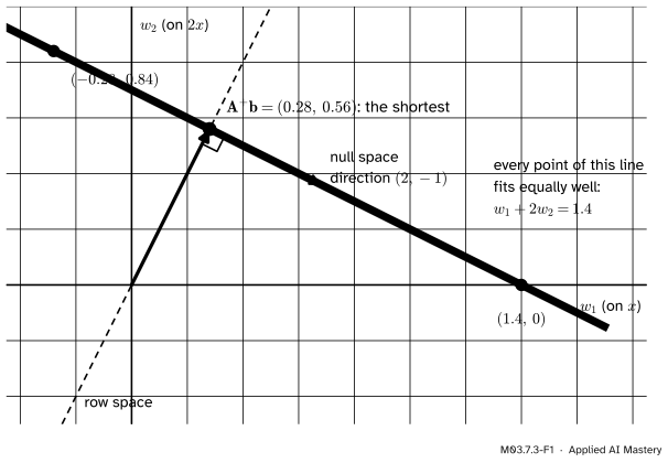
With columns \(\vect{1}\), \(\vect{x}\) and \(2\vect{x}\), the model predicts \(\hat{y} = w_0 + w_1 x + w_2 (2x)\), so only the combination \({w_1 + 2w_2}\) matters for the slope. Any pair with \(w_1 + 2w_2 = 1.4\) gives exactly the best line. Draw those pairs in the plane of \((w_1, w_2)\) and they fill a whole line.
M03.7.3-F1
All the least-squares weights for the duplicated feature lie on one line. Moving along it changes nothing the model predicts. The pseudoinverse picks the point of the line nearest the origin, where the line is crossed at a right angle.
Least squares alone cannot choose among them. A natural tie-break is to take the shortest weight vector, the one with the least \(\norm{\vect{w}}\). In the picture that is the foot of the perpendicular from the origin to the line: another right angle, this time in the space of weights. The matrix that produces this choice for every \(\vect{b}\) at once is the pseudoinverse\(\mat{A}^+\).
Build it up
Step 1. The null space is the freedom. The third column is twice the second, so \({2\cdot(\text{column 2})} - (\text{column 3}) = \vect{0}\): the vector \((0, 2, -1)\) is in the null space of \(\mat{A}\). Adding any multiple of it to the weights leaves \(\mat{A}\vect{w}\), and so every prediction, unchanged.
Step 2. All solutions are one solution plus the null space. If \(\vect{w}_1\) and \(\vect{w}_2\) are both least-squares solutions, then \(\mat{A}\vect{w}_1\) and \(\mat{A}\vect{w}_2\) are both the projection of \(\vect{b}\) onto the column space, the one closest point of lesson M03.7.1. Subtracting, \(\mat{A}(\vect{w}_1 - \vect{w}_2) = \vect{0}\): they differ by a null-space vector. Here one solution is \((0.5, 1.4, 0)\), the ML01 line, so every solution is \((0.5,\ 1.4 - 2t,\ t)\) for some number \(t\).
Step 3. The row space is where the shortest one lives. The row space of \(\mat{A}\) is perpendicular to its null space (M02.7). A solution that lies in the row space has no null-space part to shed. A solution with a null-space part is longer, by Pythagoras.
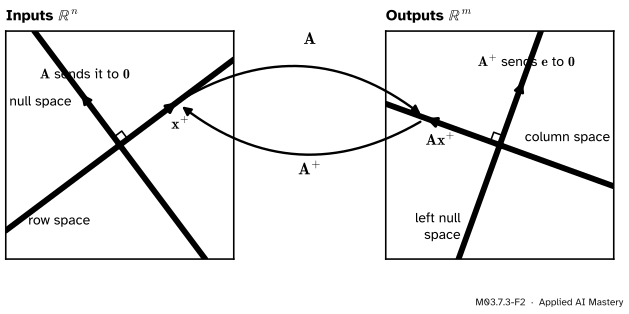
Step 4. Invert what can be inverted.\(\mat{A}\) carries the row space onto the column space one to one; only the null space is lost. So “undo \(\mat{A}\)” makes sense from the column space back to the row space, and nowhere else.
M03.7.3-F2
The four subspaces of M02.7 again. \(\mat{A}\) matches the row space with the column space one to one; \(\mat{A}^+\) runs that match backwards and sends the left null space, where the residual lives, to zero.
The formal statement
NoteDefinition: the pseudoinverse
Let \(\mat{A} = \mat{U}\mat{\Sigma}\mat{V}\T\) be the SVD of an \(m \times n\) matrix of rank \(r\), with singular values \(\sigma_1 \ge \dots \ge \sigma_r > 0\). Let \(\mat{\Sigma}^+\) be the \(n \times m\) matrix with \(1/\sigma_1, \dots, 1/\sigma_r\) on its diagonal and zeros everywhere else. The pseudoinverse (Moore–Penrose inverse) is
\(\vect{x}^+ = \mat{A}^+\vect{b}\) is a least-squares solution of \(\mat{A}\vect{x} \approx \vect{b}\), and every other least-squares solution is longer.
Proof, part 1: \(\vect{x}^+\) is a least-squares solution. Multiply out, using \(\mat{V}\T\mat{V} = \mat{I}\):
The \(m \times m\) matrix \(\mat{\Sigma}\mat{\Sigma}^+\) has ones in its first \(r\) diagonal places and zeros elsewhere, so this is \(\sum_{i \le r} {(\vect{u}_i \cdot \vect{b})}\,\vect{u}_i\). The first \(r\) columns of \(\mat{U}\) are an orthonormal basis of the column space (M03.5.3), so this sum is the projection of \(\vect{b}\) onto the column space: the closest point, as lesson M03.7.1 requires.
Part 2: every other solution is longer. By Step 2 any least-squares solution is \(\vect{x}^+ + \vect{n}\) with \(\mat{A}\vect{n} = \vect{0}\). The vector \(\vect{x}^+\) is a combination of \(\vect{v}_1, \dots, \vect{v}_r\), a basis of the row space, and \(\vect{n}\) lies in the null space, spanned by the remaining \(\vect{v}\)’s. So \(\vect{x}^+ \cdot \vect{n} = 0\), and
That exceeds \(\norm{\vect{x}^+}^2\) unless \(\vect{n} = \vect{0}\). \(\blacksquare\)
Two special cases.
Independent columns (\(r = n\)). There is only one least-squares solution, so \(\mat{A}^+\vect{b}\) equals \({(\mat{A}\T\mat{A})^{-1}\mat{A}\T\vect{b}}\) for every \(\vect{b}\), and the matrices agree: \(\mat{A}^+ = {(\mat{A}\T\mat{A})^{-1}\mat{A}\T}\), Strang’s left inverse. For the running \(\mat{B}\), \(\mat{B}^+ = \tfrac13\begin{bmatrix} 1 & 2 & -1 \\ 1 & -1 & 2 \end{bmatrix}\).
Square and invertible (\(r = m = n\)). Then \(\mat{\Sigma}^+ = \mat{\Sigma}^{-1}\) and \(\mat{A}^+ = {\mat{V}\mat{\Sigma}^{-1}\mat{U}\T} = \mat{A}^{-1}\).
The Penrose conditions. The pseudoinverse is the one and only matrix \(\mat{X}\) that satisfies all four of
The last two say that \(\mat{A}\mat{A}^+\) and \(\mat{A}^+\mat{A}\) are symmetric; in fact \(\mat{A}\mat{A}^+\) projects onto the column space (it is the hat matrix \(\mat{H}\) when the columns are independent) and \(\mat{A}^+\mat{A}\) projects onto the row space.
Go deeper: why the first condition holds
Multiply out with the SVD: \(\mat{A}\mat{A}^+\mat{A} = {\mat{U}\mat{\Sigma}\mat{\Sigma}^+\mat{\Sigma}\mat{V}\T}\). The middle product \(\mat{\Sigma}\mat{\Sigma}^+\mat{\Sigma}\) multiplies each \(\sigma_i\) by \(1/\sigma_i\) and by \(\sigma_i\) again, giving \(\sigma_i\) back for \(i \le r\), and leaves the zeros as zeros. So it is \(\mat{\Sigma}\), and \(\mat{A}\mat{A}^+\mat{A} = \mat{A}\). The second condition is the same computation with \(\mat{\Sigma}^+\mat{\Sigma}\mat{\Sigma}^+ = \mat{\Sigma}^+\). For the last two, \(\mat{A}\mat{A}^+ = {\mat{U}(\mat{\Sigma}\mat{\Sigma}^+)\mat{U}\T}\) and \(\mat{A}^+\mat{A} = {\mat{V}(\mat{\Sigma}^+\mat{\Sigma})\mat{V}\T}\) have a diagonal matrix in the middle, so they equal their transposes. That no other matrix satisfies all four is a theorem we do not prove here. The four conditions are Penrose’s, from 1955; the matrix itself had already been described by E. H. Moore in 1920 and by Arne Bjerhammar in 1951.
Worked example
The minimum-norm weights for the columns \(\vect{1}\), \(\vect{x}\), \(2\vect{x}\), by hand.
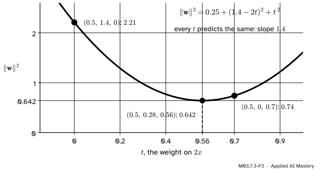
All the solutions. The ML01 line gives one solution, \((0.5, 1.4, 0)\), and the null space is spanned by \((0, 2, -1)\). So the solutions are
\[
\vect{w}(t) = (0.5,\ 1.4 - 2t,\ t) .
\]
Each predicts \(0.5 + (1.4 - 2t)\,x + t\,(2x) = 0.5 + 1.4x\): the same line for every \(t\).
so \(t = 0.56\) and \(\vect{w}^+ = (0.5,\ 1.4 - 1.12,\ 0.56) = (0.5, 0.28, 0.56)\). Its squared length is \({0.25 + 0.0784 + 0.3136} = 0.642\), against \(2.21\) for the ML01 weights \((0.5, 1.4, 0)\).
Check the right angle.\(\vect{w}^+ \cdot (0, 2, -1) = {0.56 - 0.56} = 0\): the minimum-norm solution is perpendicular to the null space, as the proof demands. The slope \(1.4\) is shared as \(0.28 + 2 \times 0.56\), in the ratio \(1 : 2\) of the two columns. The intercept, \(0.5\), is not touched, because the null-space direction has no first entry.
Code
The pseudoinverse from scratch, with a cut-off below which a singular value counts as zero.
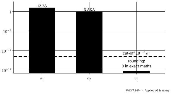
The third singular value is zero in exact arithmetic; the computer returns a speck of rounding, far below the cut-off, so it is treated as zero rather than divided by. lstsq gives the same weights (its documentation: “If there are multiple minimizing solutions, the one with the smallest 2-norm is returned”), and since the rank, 2, is below the number of columns, its residuals output is empty.
M03.7.3-F4
The singular values of the design with columns \(\vect{1}\), \(\vect{x}\), \(2\vect{x}\). Anything below the dashed cut-off is set to zero in \(\mat{\Sigma}^+\) instead of being inverted.
Now the four Penrose conditions, and the special cases.
P = pinv_from_svd(A)conditions = [np.allclose(A @ P @ A, A), np.allclose(P @ A @ P, P), np.allclose((A @ P).T, A @ P), np.allclose((P @ A).T, P @ A)]print("Penrose conditions hold:", conditions)print("A+ A =\n", np.round(P @ A, 10))B = np.array([[1.0, 1.0], [1.0, 0.0], [0.0, 1.0]])print("3 B+ =\n", np.round(3* pinv_from_svd(B), 10))T = np.array([[1.0, 1.0], [-1.0, 2.0]])print("pinv equals inv for an invertible matrix:", np.allclose(pinv_from_svd(T), np.linalg.inv(T)))
\(\mat{A}^+\mat{A}\) is not the identity: its lower corner, with entries \(0.2, 0.4, 0.4, 0.8\), is the projection onto the direction \((1, 2)/\sqrt{5}\) of the two copies, the row-space direction of the anchor figure. NumPy’s own pinv uses the same cut-off by default: singular values “less than or equal to rcond * largest_singular_value are set to zero”, with rcond\(= 10^{-15}\).
Explore
The module’s interactive is in lesson M03.7.1. There the two columns are always independent; the pseudoinverse adds nothing new until a column repeats.
Pitfalls
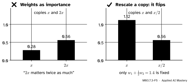
M03.7.3-F5
Wrong beside right. Scale one copy differently and the minimum-norm split flips. The split follows the sizes of the columns; it says nothing about which copy matters.
“The minimum-norm weights tell me which of the copies matters.”
They cannot: the copies carry the same information. The minimum-norm rule shares a slope among the copies in proportion to their scale, so the larger column gets the larger weight. Only the combination that the data determine, here the slope \(1.4\), has a meaning. This is why feature importances from a model with duplicated or nearly duplicated features need care.
“\(\mat{A}^+\) is always \((\mat{A}\T\mat{A})^{-1}\mat{A}\T\).”
Only when the columns are independent. With the copy \(2\vect{x}\), \(\mat{A}\T\mat{A}\) is singular (its determinant is exactly \(0\) in exact arithmetic), and np.linalg.inv(A.T @ A) either raises LinAlgError or, after rounding, returns enormous meaningless numbers. The SVD formula works for every matrix.
“\(\mat{A}^+\mat{A} = \mat{I}\), like an inverse.”
Only for independent columns. In general \(\mat{A}^+\mat{A}\) projects onto the row space and \(\mat{A}\mat{A}^+\) onto the column space; above, \(\mat{A}^+\mat{A}\) sends \((0, 1, 0)\) to \((0, 0.2, 0.4)\).
Check yourself
Recall
1. When does least squares have more than one solution, and how do the solutions differ?
Show answer
When the columns of \(\mat{A}\) are dependent. Any two solutions differ by a vector of the null space.
2. How is \(\mat{\Sigma}^+\) made from \(\mat{\Sigma}\)?
Show answer
Transpose the shape to \(n \times m\), put \(1/\sigma_i\) in place of each non-zero \(\sigma_i\), and leave the zeros as zeros.
3. Why is \(\mat{A}^+\vect{b}\) the shortest least-squares solution?
Show answer
It lies in the row space, which is perpendicular to the null space. Any other solution adds a null-space vector at a right angle, which adds to the squared length.
4. What is \(\mat{A}^+\) for a matrix with independent columns, and for an invertible matrix?
Show answer
\((\mat{A}\T\mat{A})^{-1}\mat{A}\T\), and \(\mat{A}^{-1}\).
5. What does rcond do in numpy.linalg.pinv?
Show answer
Singular values at or below rcond times the largest are set to zero instead of being inverted. The default is \(10^{-15}\).
Exercises
1.★ Find the pseudoinverse of the \(1 \times 2\) matrix \(\mat{A} = \begin{bmatrix} 1 & 2 \end{bmatrix}\) and use it to find the shortest solution of \(w_1 + 2w_2 = 1.4\).
Show solution
The rows are independent, so \(\mat{A}\mat{A}\T = 5\) is invertible and \(\mat{A}^+ = {\mat{A}\T(\mat{A}\mat{A}\T)^{-1}} = \tfrac15(1, 2)\), written as a column (Strang’s right inverse). Check with the SVD: \(\sigma_1 = \sqrt{5}\), \(\vect{u}_1 = 1\), \(\vect{v}_1 = (1, 2)/\sqrt{5}\), so \(\mat{A}^+ = {\vect{v}_1/\sigma_1} = (1, 2)/5\). Then \(\mat{A}^+(1.4) = (0.28, 0.56)\): the slope of the worked example, split in the same way.
2.★★ Find \(\mat{A}^+\) for \(\mat{A} = \begin{bmatrix} 2 & 0 \\ 0 & 0 \end{bmatrix}\) and check all four Penrose conditions.
Show solution
\(\mat{A}\) is already its own SVD with \(\mat{U} = \mat{V} = \mat{I}\) and \(\sigma = 2, 0\). So \(\mat{A}^+ = \begin{bmatrix} 0.5 & 0 \\ 0 & 0 \end{bmatrix}\). Then \(\mat{A}\mat{A}^+ = \mat{A}^+\mat{A} = \begin{bmatrix} 1 & 0 \\ 0 & 0 \end{bmatrix}\), which is symmetric (conditions 3 and 4), and
Note that \(\mat{A}\) has no inverse, and \(\mat{A}^+\mat{A} \ne \mat{I}\).
3.★★★ Prove from the thin SVD that \(\mat{A}^+ = (\mat{A}\T\mat{A})^{-1}\mat{A}\T\) when the columns of \(\mat{A}\) are independent.
Show solution
With independent columns the thin SVD has an invertible \(n \times n\) diagonal \(\mat{\Sigma}\) and a square orthogonal \(\mat{V}\), and \(\mat{A}^+ = \mat{V}\mat{\Sigma}^{-1}\mat{U}\T\). From lesson M03.7.2, \(\mat{A}\T\mat{A} = \mat{V}\mat{\Sigma}^2\mat{V}\T\), whose inverse is \(\mat{V}\mat{\Sigma}^{-2}\mat{V}\T\) (multiply the two and use \(\mat{V}\T\mat{V} = \mat{I}\)). So
When least squares has many answers, \(\mat{A}^+\) picks the shortest.
M03.7.3-F1
The foot of the perpendicular.
Definition.\(\mat{A}^+ = \mat{V}\mat{\Sigma}^+\mat{U}\T\), inverting only the non-zero \(\sigma_i\).
Solutions. All least-squares solutions are \(\mat{A}^+\vect{b} + \vect{n}\), \(\mat{A}\vect{n} = \vect{0}\).
Special cases.\((\mat{A}\T\mat{A})^{-1}\mat{A}\T\) for independent columns; \(\mat{A}^{-1}\) if invertible.
In code.np.linalg.pinv(A, rcond=1e-15); lstsq returns the same minimum-norm solution.
Sources and next steps
Sources. Each was opened and checked against this lesson on 15 November 2026.
Gilbert Strang, Left and right inverses; pseudoinverse, MIT OpenCourseWare 18.06SC, lecture 33 and its lecture summary: the left inverse \((\mat{A}\T\mat{A})^{-1}\mat{A}\T\) and right inverse \(\mat{A}\T(\mat{A}\mat{A}\T)^{-1}\), the one-to-one map from the row space to the column space, and \(\mat{A}^+ = \mat{V}\mat{\Sigma}^+\mat{U}\T\) with \(1/\sigma_1, \dots, 1/\sigma_r\) on the diagonal of \(\mat{\Sigma}^+\).
David Austin, Understanding Linear Algebra, Using Singular Value Decompositions, subsection Least-squares problems: Proposition 7.5.3, that \(\mat{V}_r\mat{\Sigma}_r^{-1}\mat{U}_r\T\vect{b}\) is the solution “of shortest length” when the columns are dependent; the definition of the Moore–Penrose pseudoinverse; and \(\mat{A}^{-1} = \mat{A}^+\) for an invertible \(\mat{A}\).
Wikipedia, Moore–Penrose inverse. The four conditions, the statement that every matrix has one and only one pseudoinverse, and its history (Moore 1920, Bjerhammar 1951, Penrose 1955).
NumPy, numpy.linalg.pinv (the cut-off rcond, default \(10^{-15}\), and its alias rtol from NumPy 2.0) and numpy.linalg.lstsq (the smallest-norm solution, and the empty residuals when the rank is below \(n\)).