The SVD of the centred data gives the principal directions, their variances and the scores in one step, without forming the covariance matrix. Derive why, decide whether to standardise, choose how many components to keep, and run PCA on the iris measurements from scratch and with scikit-learn.
M03.6.4L2 Intermediate25 minIn review (what this means)
The maths and code on this page are checked by automated tests on every change, but an independent reader has not signed it off yet. Spot a mistake or a confusing step? Tell us.
Derive from X_c = U Sigma V-transpose that the principal directions are the columns of V, the variances are sigma_i^2 / (n - 1) and the scores are U Sigma.
Explain why PCA by SVD is more accurate than PCA through the covariance matrix, and demonstrate the difference in code.
Decide when to standardise the features, and show how a change of units changes the answer.
Choose the number of components with a scree plot or a variance threshold, and read the output of sklearn.decomposition.PCA.
The question
Every data-science library has a PCA function, and none of them computes it the way the last lesson did. They skip the covariance matrix and take an SVD of the data instead. Why is that the same answer, why is it a better way to get it, and how do you read what sklearn.decomposition.PCA hands back?
From the last lesson
1. What is the variance of centred data along a unit direction \(\vect{u}\)?
Show answer
\(\vect{u}\T\mat{C}\vect{u}\), where \(\mat{C} = {\mat{X}_c\T\mat{X}_c/(n - 1)}\).
2. What is the explained-variance ratio of the \(j\)-th principal direction?
Show answer
\({\lambda_j/\operatorname{tr}(\mat{C})}\): its eigenvalue over the sum of all the eigenvalues.
Intuition
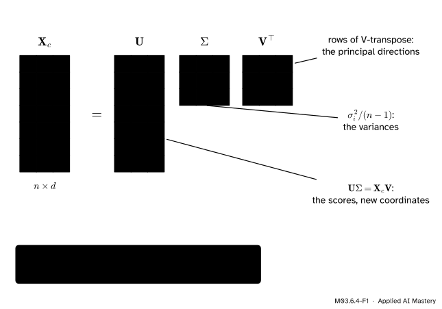
The last lesson built \(\mat{C}\) from the centred data \(\mat{X}_c\) and then took it apart again into eigenvectors. The SVD takes \(\mat{X}_c\) apart directly, and every piece of PCA is one of its factors.
M03.6.4-F1
PCA read off the SVD of the centred data: the directions from \(\mat{V}\T\), the variances from \(\mat{\Sigma}\), the new coordinates from \(\mat{U}\mat{\Sigma}\).
So PCA is one SVD. The rest of the lesson derives the three readings, explains why skipping \(\mat{C}\) is more than a shortcut, and deals with two practical questions: should the features be rescaled first, and how many directions should be kept?
Build it up
Step 1. The covariance matrix from the SVD. Take the thin SVD \(\mat{X}_c = \mat{U}\mat{\Sigma}\mat{V}\T\) (M03.5.3), with \(\mat{U}\T\mat{U} = \mat{I}\) and \(\mat{V}\) square and orthogonal. Then
This is an eigendecomposition of \(\mat{C}\): the eigenvectors are the columns \(\cparam{\vect{v}_i}\) of \(\mat{V}\), the right singular vectors, and the eigenvalues are \(\cparam{\sigma_i^2/(n - 1)}\). (The \(\vect{q}_i\) of the last lesson are these \(\vect{v}_i\); the letter \(\vect{u}\) now names the left singular vectors.)
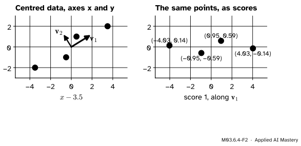
Step 2. The scores. The score of point \(i\) on direction \(j\) is \(\vect{v}_j \cdot \vect{x}_i\), so all the scores together are \(\mat{X}_c\mat{V}\), and
Column \(j\) of the scores is \(\sigma_j\vect{u}_j\). The scores are the same points, described in the principal directions instead of the original axes.
M03.6.4-F2
Scores are coordinates in the principal directions. Turned so that \(\vect{v}_1\) points along the horizontal axis, the four points lie almost on a line.
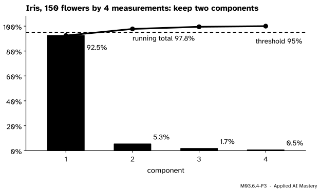
Step 3. How many components? Order the variances from largest to smallest and plot them: a scree plot. Keep the components before the curve flattens, or keep the fewest whose explained-variance ratios add up to a chosen threshold, say 95%.
M03.6.4-F3
A scree plot for the iris measurements. The first component explains 92.5% of the variance; the first two, 97.8%, clear a 95% threshold.
The formal statement
NotePCA by SVD
Let \(\mat{X}\) be an \(n \times d\) data matrix, one row per item, with column means removed to give \(\mat{X}_c\), and let \(\mat{X}_c = \mat{U}\mat{\Sigma}\mat{V}\T\) be its thin SVD. Then
the principal directions are the columns \(\vect{v}_1, \dots, \vect{v}_d\) of \(\mat{V}\);
the variance along \(\vect{v}_j\) is \(\sigma_j^2/(n - 1)\), and its explained-variance ratio is \({\sigma_j^2/(\sigma_1^2 + \cdots + \sigma_d^2)}\);
the scores are \(\mat{X}_c\mat{V} = \mat{U}\mat{\Sigma}\).
Keeping \(k\) components is the best rank-\(k\) approximation. Project every point onto the first \(k\) directions and map back: the reconstruction is \(\mat{X}_c\mat{V}_k\mat{V}_k\T\), where \(\mat{V}_k\) holds the first \(k\) columns. Since \(\mat{V}\T\mat{V}_k\) is the first \(k\) columns of the identity, \(\mat{X}_c\mat{V}_k = \mat{U}_k\mat{\Sigma}_k\), and
That is the truncation of the SVD. By the Eckart-Young theorem (M03.6.1) no other rank-\(k\) matrix is closer to the data, and the squared error is \({\sigma_{k+1}^2 + \cdots + \sigma_d^2}\), which is \(n - 1\) times the variance left out.
Why the SVD is more accurate. Forming \(\mat{X}_c\T\mat{X}_c\) squares the singular values. A small \(\sigma_d\) next to a large \(\sigma_1\) becomes a far smaller \(\sigma_d^2\) next to \(\sigma_1^2\), and a computer that keeps about 16 significant digits loses the small one entirely once \(\sigma_1/\sigma_d\) passes about \(10^8\). The SVD works on \(\mat{X}_c\) itself and keeps it. M03.8.2 gives the reason a name: the condition number of \(\mat{X}_c\T\mat{X}_c\) is the square of that of \(\mat{X}_c\).
Standardising. PCA compares variances, and a variance carries the square of the units. Measure one feature in millimetres instead of centimetres and its variance grows a hundredfold, so it takes over the first component. When the features are in different units, or on very different scales, divide each centred column by its standard deviation first. PCA of these standardised features is PCA of the correlation matrix (M06.10.3), and it does not depend on the units.
Worked example
The running four points, by SVD. Take \(\vect{v}_1 = {(1, 0.618)/1.176} \approx (0.851, 0.526)\), the direction of slope \({(\sqrt5 - 1)/2}\) from the last lesson. Each score is one row of \(\mat{X}_c\) dotted with \(\vect{v}_1\); for the first point, \({-3.5 \times 0.851} - {2 \times 0.526} \approx -4.03\). All four together:
In exact form \(\sigma_1^2 = {(35 + 15\sqrt5)/2}\), and since \({(2.5 + 1.5\sqrt5)^2} = {6.25 + 11.25 + 7.5\sqrt5}\), which is the same number, \(\sigma_1 = 2.5 + 1.5\sqrt5 \approx 5.854\). Likewise \(\sigma_2 = 1.5\sqrt5 - 2.5 \approx 0.854\). Dividing their squares by \(n - 1 = 3\) gives the variances \(11.42\) and \(0.24\) of the last lesson, and no covariance matrix was needed once the direction was known.
Standardised. The standard deviations of the two columns are \(\sqrt{25/3}\) and \(\sqrt{10/3}\), so the correlation matrix has \(r = {15/\sqrt{25 \cdot 10}} = {3/\sqrt{10}} \approx 0.949\) off the diagonal. Its eigenvectors are \({(1, 1)/\sqrt2}\) and \({(1, -1)/\sqrt2}\) with eigenvalues \(1 + r\) and \(1 - r\) (exercise 3), so after standardising, the first component explains \({(1 + r)/2} \approx 97.4\%\). The direction has changed from slope \(0.618\) to slope 1 in the standardised units.
Code
From scratch: PCA by SVD on the iris measurements, 150 flowers by 4 lengths in centimetres.
import numpy as npfrom sklearn.datasets import load_irisX = load_iris().datan =len(X)Xc = X - X.mean(axis=0)U, s, Vt = np.linalg.svd(Xc, full_matrices=False)variances = s **2/ (n -1)ratios = variances / variances.sum()scores = U * s # the same as Xc @ Vt.Tprint("variances:", variances.round(4))print("ratios:", ratios.round(4), " running total:", np.cumsum(ratios).round(4))print("first direction:", Vt[0].round(3))k =int(np.argmax(np.cumsum(ratios) >=0.95)) +1print("components needed for 95%:", k)
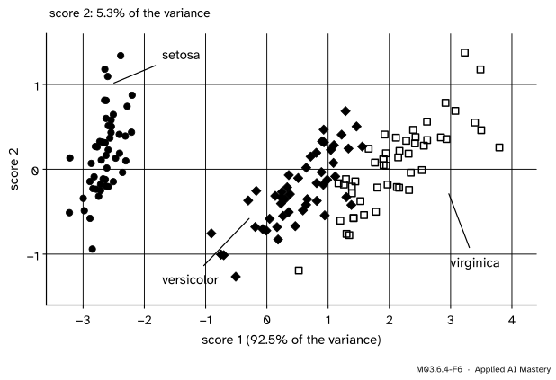
The first direction leans mostly on petal length (0.857). The projection onto two components is the next picture.
M03.6.4-F6
Four measurements drawn in two dimensions. Setosa stands apart along the first component; the other two species overlap.
scikit-learn’s PCA centres the data (but does not scale it) and returns the same numbers. Its components_ are the rows of \(\mat{V}\T\), possibly with other signs, and explained_variance_ is \(\sigma_i^2/(n - 1)\).
from sklearn.decomposition import PCApca = PCA(n_components=2).fit(X)print("components_:\n", pca.components_.round(3))print("explained_variance_:", pca.explained_variance_.round(4))print("explained_variance_ratio_:", pca.explained_variance_ratio_.round(4))signs = np.sign(np.sum(pca.components_ * Vt[:2], axis=1)) # +1 or -1 for each directionprint("same directions up to sign:", np.allclose(pca.components_, signs[:, None] * Vt[:2]))print("same scores up to sign:", np.allclose(pca.transform(X), scores[:, :2] * signs))
components_:
 [[ 0.361 -0.085  0.857  0.358]
 [ 0.657  0.73  -0.173 -0.075]]
explained_variance_: [4.2282 0.2427]
explained_variance_ratio_: [0.9246 0.0531]
same directions up to sign: True
same scores up to sign: True
Last, accuracy. Forty points lie almost exactly on the line \(y = x\): the second feature is the first plus \(10^{-8}\) times a pattern perpendicular to it. The true small variance is about \(5.1 \times 10^{-17}\). By default scikit-learn’s PCA forms the covariance matrix when there are many more rows than columns (its svd_solver="auto" rule); svd_solver="full" uses the SVD.
t = np.tile([-3.0, -1.0, 1.0, 3.0], 10)pattern = np.tile([1.0, -1.0, -1.0, 1.0], 10) # perpendicular to t, and adds up to zeroZ = np.column_stack([t, t +1e-8* pattern]) +5.0true_small =20*1e-16/39# 20 times delta squared, over n - 1 (to 16 digits)through_C = np.linalg.eigvalsh(np.cov(Z, rowvar=False))[0]by_svd = np.linalg.svd(Z - Z.mean(axis=0), compute_uv=False)[1] **2/39default = PCA().fit(Z).explained_variance_[1]full = PCA(svd_solver="full").fit(Z).explained_variance_[1]for name, value in [("through C", through_C), ("by SVD", by_svd), ("PCA default", default), ("PCA full", full)]:print(f"{name:12s}{value: .3e} relative error {abs(value - true_small) / true_small:.1e}")
through C     1.583e-15   relative error 3.0e+01
by SVD        5.128e-17   relative error 5.9e-08
PCA default   6.263e-16   relative error 1.1e+01
PCA full      5.128e-17   relative error 5.9e-08
The two routes through the covariance matrix return rounding noise; the two SVD routes are right to several digits.
Explore
The module’s interactive, the rank slider, is in lesson M03.6.2. Read its bars as a scree plot: the square of each bar over \(n - 1\) would be the variance of one component, and the share of the energy kept plays the part of the explained-variance ratio. (The picture is not centred, which is why its first bar is so tall.)
Pitfalls
M03.6.4-F5
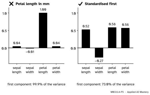
Wrong beside right. Record one feature in millimetres and the first component is that feature alone. Standardised, all four features have a say.
“PCA does not care about units.”
It does, because it compares variances. With petal length in millimetres the first component of iris is \((0.04, -0.01, 1.00, 0.04)\) and explains 99.9% of the variance: it has found the column with the largest numbers, nothing more. Standardise when the units differ. When they are all the same, as in centimetres for iris, standardising is a choice, and it changes the answer (92.5% becomes 73.0%).
“My components have the opposite signs to the library’s, so one of us is wrong.”
If \(\vect{v}_j\) is a principal direction, so is \(-\vect{v}_j\), with the matching \(\vect{u}_j\) flipped too; \(\mat{U}\mat{\Sigma}\mat{V}\T\) does not change. Compare directions up to sign, as the code does, and never read meaning into the sign of a component alone.
“explained_variance_ holds the singular values.”
It holds \(\sigma_i^2/(n - 1)\), the variances. The singular values themselves are in singular_values_, and the ratios in explained_variance_ratio_. Mixing them up changes a scree plot’s shape: singular values fall more slowly than their squares.
Check yourself
Recall
1. In \(\mat{X}_c = \mat{U}\mat{\Sigma}\mat{V}\T\), where are the principal directions?
Show answer
In the columns of \(\mat{V}\), the rows of \(\mat{V}\T\).
2. What is the variance along the \(j\)-th principal direction, in terms of the SVD?
Show answer
\(\sigma_j^2/(n - 1)\).
3. What are the scores, and why do they equal \(\mat{U}\mat{\Sigma}\)?
Show answer
The coordinates of the points in the principal directions, \(\mat{X}_c\mat{V}\). Since \(\mat{V}\T\mat{V} = \mat{I}\), \(\mat{X}_c\mat{V} = \mat{U}\mat{\Sigma}\mat{V}\T\mat{V} = \mat{U}\mat{\Sigma}\).
4. Why is the SVD of \(\mat{X}_c\) more accurate than the eigenvectors of \(\mat{C}\)?
Show answer
Forming \(\mat{X}_c\T\mat{X}_c\) squares the singular values, so a small one beside a large one can fall below the rounding of the large one and be lost. The SVD works on \(\mat{X}_c\) itself.
5. When should the features be standardised before PCA?
Show answer
When they are measured in different units or on very different scales; otherwise the feature with the largest numbers dominates the first component.
Exercises
1.★ Centred data with \(n = 10\) rows have singular values 6 and 3. Find the variances along the principal directions and the explained-variance ratios.
Show solution
The variances are \({36/9} = 4\) and \({9/9} = 1\). The ratios are \(36/45 = 80\%\) and \(9/45 = 20\%\).
2.★★ Show that the scores on different principal directions are uncorrelated, and that the variance of the scores on direction \(j\) is \(\sigma_j^2/(n - 1)\).
Show solution
The scores are the columns of \(\mat{U}\mat{\Sigma}\), and each adds up to zero because the columns of \(\mat{X}_c\) do. Their covariance matrix is
which is diagonal. The zeros off the diagonal say that the scores are uncorrelated, and the diagonal holds the variances \(\sigma_j^2/(n - 1)\).
3.★★★ Two standardised features have correlation \(r > 0\). Show that their principal directions are always \({(1, 1)/\sqrt2}\) and \({(1, -1)/\sqrt2}\), find the explained-variance ratio of the first, and evaluate it for the running four points.
Show solution
Standardised features have variance 1, so their covariance matrix is the correlation matrix \(\mat{R} = \begin{bmatrix} 1 & r \\ r & 1 \end{bmatrix}\). Multiplying,
so the directions are \({(1, 1)/\sqrt2}\) and \({(1, -1)/\sqrt2}\) whatever \(r\) is, with variances \(1 + r\) and \(1 - r\). With \(r > 0\) the first is the larger, and its ratio is \({(1 + r)/2}\). For the running points \(r = 3/\sqrt{10} \approx 0.949\), so the ratio is about \(97.4\%\).
Summary card
One SVD of the centred data is a whole PCA.
M03.6.4-F1
Directions, variances, scores.
Directions. The columns of \(\mat{V}\) in \(\mat{X}_c = \mat{U}\mat{\Sigma}\mat{V}\T\).
In practice. Centre always, standardise when units differ, and keep components until a scree plot flattens or a threshold is met.
Sources and next steps
Sources. Each was opened and checked against this lesson on 15 November 2026.
Marc Deisenroth, Aldo Faisal and Cheng Soon Ong, Mathematics for Machine Learning, Section 10.4. Equations (10.47) to (10.49): with the data in the columns of \(\mat{X}\), the eigenvectors of the covariance matrix are the left singular vectors of \(\mat{X}\) and its eigenvalues are \(\sigma_d^2/N\); Section 10.4.1 links PCA to the Eckart-Young theorem. Section 10.6 lists the steps of PCA in practice: subtract the mean, then divide each dimension by its standard deviation.
David Austin, Understanding Linear Algebra, Using singular value decompositions, subsection “Principal component analysis”: the principal components are the left singular vectors of the demeaned data matrix, which stores points as columns, and the variance in the direction of \(\vect{u}_i\) is \(\sigma_i^2/N\).
scikit-learn, PCA (version 1.9.1). The input “is centered but not scaled”; explained_variance_ uses n_samples - 1 degrees of freedom; components_ are the right singular vectors of the centred data; the “auto” solver uses "covariance_eigh" when there are fewer than 1,000 features and more than 10 times as many samples, a solver that “effectively doubles the condition number and is therefore less numerical stable”. load_iris gives the 150 by 4 iris measurements.
NumPy, numpy.linalg.svd: the rows of Vh are the eigenvectors of \(\mat{A}\T\mat{A}\), that is the right singular vectors, and the singular values come in descending order.