A greyscale picture is a matrix, so the truncated SVD compresses it. Count what k layers cost to store, watch how fast a photograph’s singular values fall, choose k by the share of the energy kept, and see why noise refuses to compress.
M03.6.2L2 Intermediate25 minIn review (what this means)
The maths and code on this page are checked by automated tests on every change, but an independent reader has not signed it off yet. Spot a mistake or a confusing step? Tell us.
Count the numbers needed to store k layers of an m by n picture, k(m + n + 1), and find the largest k that still saves space.
Choose k from the share of the energy kept, and convert that share into a relative error.
Compress a photograph with numpy.linalg.svd and with sklearn.decomposition.TruncatedSVD, and compare the two.
Explain why sharp slanted edges, fine texture and noise need many layers.
The question
A greyscale photograph 427 pixels high and 640 wide is a table of 273,280 brightness values. Keep only its first 50 singular layers and you store a fifth as many numbers. How much of the picture survives, how should you choose how many layers to keep, and why do some pictures refuse to be squeezed at all?
From the last lesson
1. What is the squared Frobenius error of the truncation \(\mat{A}_k\)?
Show answer
The sum of the squares of the dropped singular values, \({\sigma_{k+1}^2 + \cdots + \sigma_r^2}\).
2. Is there a matrix of rank \(k\) that is closer to \(\mat{A}\) than \(\mat{A}_k\)?
Show answer
No. By the Eckart-Young theorem no matrix of rank at most \(k\) is closer, in the Frobenius or the spectral norm.
Intuition
A greyscale picture is a grid of pixels, each with a brightness from 0 (black) to 1 (white). Read the grid row by row and it is a matrix. This module draws its own small one: a house, a hill and the sun on a \(48 \times 48\) grid.
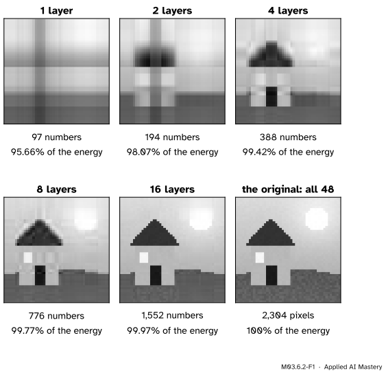
By the last lesson, the best rank-\(k\) copy of that matrix is its first \(k\) singular layers. So rebuild the picture from 1 layer, then 2, then 4, and so on.
M03.6.2-F1
The module’s picture rebuilt from its first \(k\) layers. Each layer costs 97 numbers. Eight layers cost a third of the 2,304 pixels and already show every object.
Broad shapes come first, because they carry most of the brightness. Edges and texture come later. The rest of the lesson puts numbers on both sides of that trade: what each layer costs, and what it buys.
Build it up
Step 1. A photograph as a matrix. scikit-learn ships a colour photograph of a Chinese temple, load_sample_image('china.jpg'), as an array of 427 rows, 640 columns and 3 colour channels. Averaging the three channels and dividing by 255 gives a greyscale matrix \(\mat{A}\) of size \(427 \times 640\) with entries between 0 and 1. (We keep the photograph itself off this page, because the site draws all its own pictures. The code below works with its numbers.)
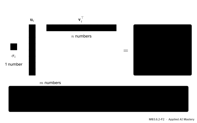
Step 2. What a layer costs. A layer \({\sigma_i\,\vect{u}_i\vect{v}_i\T}\) fills a whole \(m \times n\) grid, but to store it you need only \(\vect{u}_i\) (\(m\) numbers), \(\vect{v}_i\) (\(n\) numbers) and \(\sigma_i\) (one number).
M03.6.2-F2
One layer is built from \(m + n + 1\) stored numbers. The picture itself needs \(mn\).
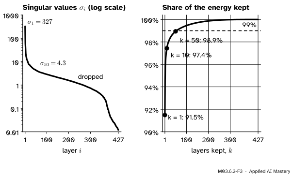
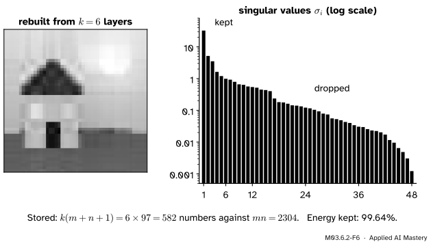
Step 3. How fast the singular values fall. For the photograph, \(\sigma_1 \approx 327\), but \(\sigma_{50}\) is already down to about 4, and the last ones are below 0.1. Since the energy is the sum of the \(\sigma_i^2\), a handful of layers holds almost all of it.
M03.6.2-F3
The singular values of the photograph fall by a factor of about 75 in the first 50 layers. The share of the energy kept rises steeply, then crawls.
The formal statement
Storage. Keeping \(k\) layers of an \(m \times n\) matrix stores \({k(m + n + 1)}\) numbers in place of \(mn\), a fraction
\[
\frac{k\,(m + n + 1)}{mn} .
\]
It saves space only while \({k(m + n + 1)} < mn\), that is while \(k < \dfrac{mn}{m + n + 1}\). For the photograph that bound is \(273{,}280/1{,}068 \approx 255.9\): up to 255 layers save space. For the \(48 \times 48\) picture it is \(2{,}304/97 \approx 23.8\).
Energy kept and error. By Result 2 of the last lesson, the squared error of \(\mat{A}_k\) is the energy that was dropped. Divide by the whole energy \(\norm{\mat{A}}_F^2\):
So the relative error\(\norm{\mat{A} - \mat{A}_k}_F / \norm{\mat{A}}_F\) is the square root of the share dropped. Keeping 99% of the energy means a relative error of \(\sqrt{0.01} = 10\%\).
Choosing \(k\). Pick a share \(s\), say 99%, and take the smallest \(k\) whose layers hold at least that share of the energy. For the photograph that is a little over 50 layers.
Why must the share be set so high? The first layer is large because a picture is mostly of one overall brightness. A flat grey picture whose every pixel has the average brightness \(b\) of the photograph would be the rank-one matrix \({b\,\vect{1}\vect{1}\T}\), and it alone would hold 74% of the photograph’s energy. So a share of 90% says almost nothing about detail; the information is in the last few per cent.
Worked example
A square frame. The \(4 \times 4\) picture with ones round the edge and zeros inside is
This is \(\lambda\vect{w}\) when \({2 + 2t} = \lambda\) and \(2 = \lambda t\). Substituting \(t = 2/\lambda\) into the first gives \(\lambda^2 - 2\lambda - 4 = 0\), so \(\lambda = 1 \pm \sqrt5\). The larger, \(\sigma_1 = 1 + \sqrt5 \approx 3.236\), has \(t = {2/(1 + \sqrt5)} = {(\sqrt5 - 1)/2} \approx 0.618\). The other, \(1 - \sqrt5\), is negative, so \(\sigma_2 = \sqrt5 - 1 \approx 1.236\) (M03.5.4). Check: \(\sigma_1^2 + \sigma_2^2 = 12\), the energy.
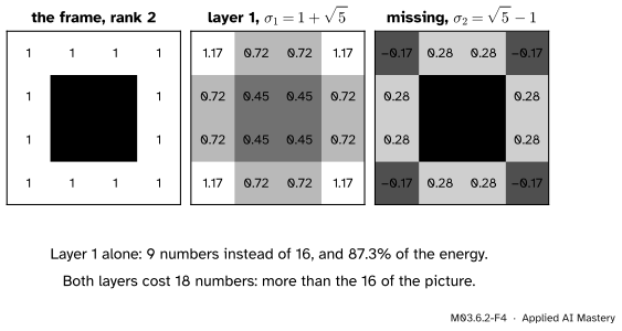
With \(\vect{u}_1 = \vect{v}_1 = \vect{w}/\norm{\vect{w}}\) and \(\norm{\vect{w}}^2 = 2 + 2t^2 = 5 - \sqrt5\), the first layer is \({\sigma_1\,\vect{w}\vect{w}\T / (5 - \sqrt5)}\). Its entries are \(1.17\) in the corners, \(0.72\) along the edges and \(0.45\) in the middle.
M03.6.2-F4
The frame, its first layer and what that layer misses. One layer blurs the frame into a soft square. The second layer, which costs as much again, puts the hole back.
The bookkeeping. One layer stores \({4 + 4 + 1} = 9\) numbers in place of 16 and keeps \({\sigma_1^2/12} = {(6 + 2\sqrt5)/12} \approx 87.3\%\) of the energy, a relative error of \(\sqrt{0.127} \approx 36\%\). Two layers rebuild the frame exactly but cost 18 numbers: here the bound \(16/9 \approx 1.8\) says that only one layer saves space.
Code
The photograph, from scratch with NumPy: its singular values, the storage and the energy kept.
import numpy as npfrom sklearn.datasets import load_sample_imageA = load_sample_image("china.jpg").mean(axis=2) /255# greyscale, entries from 0 to 1m, n = A.shapeU, s, Vt = np.linalg.svd(A, full_matrices=False)share = np.cumsum(s **2) / np.sum(s **2)print("shape:", A.shape, " sigma_1:", round(s[0], 1), " sigma_50:", round(s[49], 2))for k in (1, 10, 50, 100): stored = k * (m + n +1)print(f"k = {k:3d}: {stored:7,d} numbers ({stored / (m * n):5.1%}),"f" energy kept {share[k -1]:.2%}, relative error {np.sqrt(1- share[k -1]):.1%}")print("largest k that saves space:", (m * n) // (m + n +1))print("smallest k keeping 99% of the energy:", int(np.argmax(share >=0.99)) +1)print("a flat picture of the mean brightness holds", round(m * n * A.mean() **2/ np.sum(A **2), 2))
shape: (427, 640)   sigma_1: 327.2   sigma_50: 4.34
k =   1:   1,068 numbers ( 0.4%), energy kept 91.49%, relative error 29.2%
k =  10:  10,680 numbers ( 3.9%), energy kept 97.43%, relative error 16.0%
k =  50:  53,400 numbers (19.5%), energy kept 98.94%, relative error 10.3%
k = 100: 106,800 numbers (39.1%), energy kept 99.46%, relative error 7.4%
largest k that saves space: 255
smallest k keeping 99% of the energy: 54
a flat picture of the mean brightness holds 0.74
The relative error of 10% at \(k = 50\) comes from the formula, and the last assertion checks it against the rebuilt matrix directly.
scikit-learn’s TruncatedSVD computes only the first \(k\) layers, by a randomised method. Its fit_transform returns \(\mat{U}_k\mat{\Sigma}_k\) (one row per image row) and inverse_transform multiplies back by \(\mat{V}_k\T\).
from sklearn.decomposition import TruncatedSVDsvd50 = TruncatedSVD(n_components=50, random_state=0)scores = svd50.fit_transform(A) # 427 by 50: U_k times Sigma_krebuilt = svd50.inverse_transform(scores) # back to 427 by 640print("largest relative gap in sigma_1..sigma_50:", round(np.max(np.abs(svd50.singular_values_ - s[:50]) / s[:50]), 4))print("relative error, randomised:", round(np.linalg.norm(A - rebuilt) / np.linalg.norm(A), 4)," exact:", round(np.sqrt(1- share[49]), 4))
largest relative gap in sigma_1..sigma_50: 0.0113
relative error, randomised: 0.1029   exact: 0.1028
The randomised singular values are within a few per cent of the exact ones, and its rebuilt picture is a hair worse than \(\mat{A}_{50}\): by Eckart-Young, no rank-50 matrix can be better.
Explore
M03.6-X1
Rank slider
Drag the slider, or press and drag on the bars, to keep \(k\) layers. Find the \(k\) at which the roof stops looking like a staircase of stripes, then press “What is missing” to see where the error lives. Note the \(k\) at which storage passes the 2,304 pixels.
Pitfalls
M03.6.2-F5
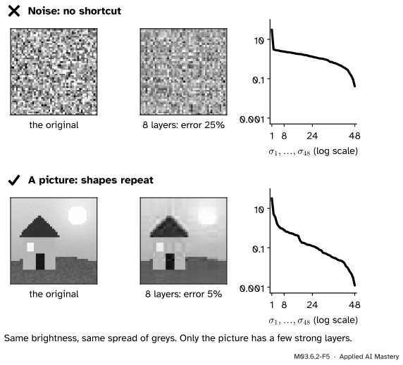
Wrong beside right. Noise with the same average and spread of greys as the picture keeps an error of 25% after 8 layers; the picture is down to 5%.
“Every image can be compressed by low rank.”
Only images whose rows repeat each other’s patterns. In random noise no row predicts another, so after the first layer, which holds the average brightness, the singular values fall slowly and evenly, with no small group of strong layers. For the noise of the figure \(\sigma_2 \approx 3.05\) and \(\sigma_9 \approx 2.28\), so each layer buys little more than the next. Sharp slanted edges are hard too: a single diagonal line of white pixels on black is the identity matrix, whose singular values are all 1, so no layer matters more than another.
“99% of the energy kept means the picture is 99% right.”
The share is of squared sizes, and most of it is plain brightness: a flat grey picture would already hold 74% of the photograph’s energy. The honest number is the relative error, the square root of the share dropped. At 99% kept it is 10%.
“Keeping more layers always saves space, just less of it.”
Past \(mn/(m + n + 1)\) layers the factors cost more than the pixels. For the \(4 \times 4\) frame that happens at the second layer, for the \(48 \times 48\) picture at the 24th, for the photograph at the 256th.
Check yourself
Recall
1. How many numbers does it take to store \(k\) layers of an \(m \times n\) picture?
Show answer
\(k(m + n + 1)\): for each layer, the \(m\) entries of \(\vect{u}_i\), the \(n\) entries of \(\vect{v}_i\) and the number \(\sigma_i\).
2. Up to which \(k\) does truncation save space?
Show answer
While \(k(m + n + 1) < mn\), that is for \(k < mn/(m + n + 1)\).
3. How do you turn the share of the energy kept into a relative error?
Show answer
The relative error \(\norm{\mat{A} - \mat{A}_k}_F/\norm{\mat{A}}_F\) is the square root of \(1 - \text{share kept}\).
4. Why does the first layer of a photograph hold so much of the energy?
Show answer
Because most of a picture’s energy is its overall brightness, and a picture of constant brightness is a rank-one matrix. The first layer captures that and little detail.
5. What does TruncatedSVD(n_components=k).fit_transform(A) return?
Show answer
The \(m \times k\) matrix \(\mat{U}_k\mat{\Sigma}_k\), computed by a randomised method; inverse_transform multiplies it by \(\mat{V}_k\T\) to give (close to) \(\mat{A}_k\).
Exercises
1.★ A greyscale picture is \(1{,}000 \times 2{,}000\). How many numbers do 100 layers cost, what fraction of the picture is that, and what is the largest \(k\) that saves space?
Show solution
One layer costs \({1{,}000 + 2{,}000 + 1} = 3{,}001\) numbers, so 100 layers cost \(300{,}100\). The picture has \(2{,}000{,}000\) pixels, so the fraction is about \(15\%\). Space is saved while \(3{,}001\,k < 2{,}000{,}000\), that is \(k < 666.4\): up to 666 layers.
2.★★ A picture of a single white diagonal line on black is the \(n \times n\) identity matrix. What share of the energy does \(\mat{A}_k\) keep, and what is the relative error? Is \(\mat{A}_k\) unique?
Show solution
\(\mat{I} = \mat{I}\,\mat{I}\,\mat{I}\T\) is an SVD, so all \(n\) singular values are 1 and the energy is \(n\). Any \(k\) layers keep \(k/n\) of it, and the relative error is \(\sqrt{1 - k/n}\): for \(n = 48\) and \(k = 8\), about \(91\%\). Because \(\sigma_k = \sigma_{k+1}\), there is a tie, and \(\mat{A}_k\) is not unique: any \(k\) orthonormal directions do equally well.
3.★★★ A picture has brightness \(b_{ij} = f_i + g_j\): a shading down the rows plus a shading across the columns. Show that its rank is at most 2, and find two layers that build it.
Show solution
Let \(\vect{f} = (f_1, \dots, f_m)\), \(\vect{g} = (g_1, \dots, g_n)\), and let \(\vect{1}\) be a vector of ones of the right length. Entry \((i, j)\) of \({\vect{f}\,\vect{1}\T}\) is \(f_i\), and entry \((i, j)\) of \({\vect{1}\,\vect{g}\T}\) is \(g_j\). So
a sum of two rank-one matrices. Its column space lies in the span of \(\vect{f}\) and \(\vect{1}\), so its rank is at most 2. These two layers are not perpendicular in general, so they are not the SVD layers, but they show that two singular values are enough: \(\sigma_3 = \sigma_4 = \cdots = 0\). The sky of the module’s picture, a gentle shading from top to bottom, is this kind of picture.
Summary card
Keep a few layers, store a few numbers, lose a little energy.
M03.6.2-F1
Broad shapes first, edges later.
Storage.\(k\) layers cost \(k(m + n + 1)\) numbers against \(mn\).
Break-even. It saves space only for \(k < mn/(m + n + 1)\).
Energy kept.\({(\sigma_1^2 + \cdots + \sigma_k^2)}/{(\sigma_1^2 + \cdots + \sigma_r^2)}\).
Sources. Each was opened and checked against this lesson on 15 November 2026.
Marc Deisenroth, Aldo Faisal and Cheng Soon Ong, Mathematics for Machine Learning, Section 4.6. The Stonehenge example: a \(1{,}432 \times 1{,}910\) greyscale image, whose rank-5 approximation needs only \({5 \cdot (1{,}432 + 1{,}910 + 1)} = 16{,}715\) numbers, “just above 0.6% of the original”: the storage count of this lesson.
scikit-learn, load_sample_image: china.jpg is returned as an array of shape \((427, 640, 3)\) and type uint8; and TruncatedSVD: it does not centre the data, its default solver is the randomised algorithm with n_iter=5, and components_ holds the right singular vectors.
NumPy, numpy.linalg.svd: full_matrices=False returns the thin factors, and the singular values come in descending order.