Cut the singular value decomposition after k layers and you have the closest matrix of rank k. Derive the error, in the Frobenius and the spectral norm, from the singular values you dropped, and test the Eckart-Young theorem against random rivals.
M03.6.1L2 Intermediate25 minIn review (what this means)
The maths and code on this page are checked by automated tests on every change, but an independent reader has not signed it off yet. Spot a mistake or a confusing step? Tell us.
Form the truncation A_k of a matrix from the first k layers of its singular value decomposition.
Derive that the squared Frobenius error of A_k is the sum of the squared singular values that were dropped, and that its spectral error is the first dropped singular value.
State the Eckart-Young theorem and explain why zeroing small entries or truncating an eigendecomposition does worse.
Build A_k in NumPy and check that random matrices of the same rank are never closer.
The question
A matrix with a million entries costs a million numbers to store. Recommender systems, compressed neural networks and the fine-tuning method LoRA all replace such a matrix by one of low rank, which costs far fewer. Of all the matrices of rank \(k\), which one is closest to the original, and how close can it possibly get?
Intuition
The last module wrote every matrix as a stack of rank-one layers, one per singular value (M03.5.4):
The layers come in order of size, \(\sigma_1 \ge \sigma_2 \ge \cdots \ge \sigma_r > 0\). The obvious way to save space is to keep the big layers and throw away the small ones. The truncation\(\cmodel{\mat{A}_k}\) is the sum of the first \(k\) layers. Each layer is a column times a row, so it has rank one, and \(\mat{A}_k\) has rank \(k\).
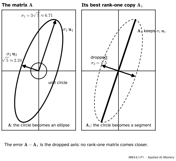
Picture what that does for the running SVD matrix \(\mat{A} = \begin{bmatrix} 3 & 0 \\ 4 & 5 \end{bmatrix}\). It turns the unit circle into an ellipse with semi-axes \(\sigma_1 = 3\sqrt5\) and \(\sigma_2 = \sqrt5\). Keeping one layer squashes the ellipse flat onto its long axis.
M03.6.1-F1
Keeping one layer of \(\mat{A}\) keeps the long axis of its ellipse and squashes the short one to nothing. What is lost is exactly the short axis, of length \(\sigma_2\).
Two claims hide in this picture. The size of the error is set by the dropped singular value alone. And nothing of rank one does better. This lesson proves the first and states the second, the Eckart-Young theorem, with its proof in a collapsed block.
Build it up
Step 1. Two ways to measure an error. To say how close \(\mat{A}_k\) is, we need the size of the error matrix \(\mat{A} - \mat{A}_k\). Two sizes are in common use, and M03.5.4 met both.
The Frobenius norm treats a matrix as a long list of entries: \(\norm{\mat{M}}_F\) is the square root of the sum of the squares of all the entries.
The spectral norm\(\norm{\mat{M}}_2\) is the largest stretch, the biggest value of \(\norm{\mat{M}\vect{x}}\) over unit vectors \(\vect{x}\).
M03.8.1 studies norms of matrices in full. Here we need only these two.
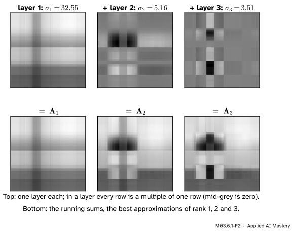
Step 2. Layer by layer. Adding layers one at a time rebuilds the matrix in order of importance. The figure shows it on a \(48 \times 48\) greyscale picture, a matrix of brightness values that the next lesson compresses.
M03.6.1-F2
Layers of a picture and their running sums. Each layer is a plaid of stripes, because every row of a rank-one matrix is a multiple of one row. Their sums \(\mat{A}_1, \mat{A}_2, \mat{A}_3\) sharpen step by step.
Step 3. The error is the layers you left out. Subtract the truncation from the full sum and what remains is the tail:
The next section measures this tail in both norms.
The formal statement
Result 1: the layers are perpendicular. Treat matrices of one shape as long vectors and define their dot product entry by entry, \(\langle \mat{X}, \mat{Y} \rangle = \sum_{a,b} x_{ab}\,y_{ab}\), so that \(\norm{\mat{X}}_F^2 = \langle \mat{X}, \mat{X} \rangle\). Entry \((a, b)\) of the layer \(\vect{u}_i\vect{v}_i\T\) is \((u_i)_a\,(v_i)_b\). So
The \(\vect{u}\)’s are orthonormal and so are the \(\vect{v}\)’s. The product is 1 when \(i = j\) and 0 otherwise: the layers are orthonormal, like the axes of a coordinate system.
Result 2: the Frobenius error. Expand the squared norm of the tail as a double sum of dot products. By Result 1 only the terms with \(i = j\) survive:
With \(k = 0\) the same line gives \(\norm{\mat{A}}_F^2 = {\sigma_1^2 + \cdots + \sigma_r^2}\): the sum of the squares of the entries equals the sum of the squared singular values. We call that sum the energy of the matrix. The share of the energy that \(\mat{A}_k\) keeps is \({\sigma_1^2 + \cdots + \sigma_k^2}\) divided by the whole sum.
Result 3: the spectral error. Take a unit vector \(\vect{x}\). Each layer acts by \({(\vect{u}_i\vect{v}_i\T)\,\vect{x}} = {(\vect{v}_i \cdot \vect{x})\,\vect{u}_i}\), so
The \(\vect{u}_i\) are orthonormal, so the squared length is the sum of the squared coefficients. Every \(\sigma_i\) in the tail is at most \(\sigma_{k+1}\), and the squared coordinates of \(\vect{x}\) along orthonormal directions add up to at most \(\norm{\vect{x}}^2 = 1\):
For \(\vect{x} = \vect{v}_{k+1}\) both inequalities are equalities. So \(\norm{\mat{A} - \mat{A}_k}_2 = \closs{\sigma_{k+1}}\), the largest singular value left out. (When \(k = r\) nothing is left out and the error is zero.)
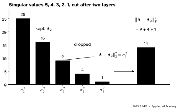
M03.6.1-F3
A matrix with singular values 5, 4, 3, 2, 1, cut after two layers. The squared spectral error is the tallest dropped bar, \(\sigma_3^2 = 9\). The squared Frobenius error is all the dropped bars stacked, \(9 + 4 + 1 = 14\).
NoteThe Eckart-Young theorem
Let \(\mat{A}\) have singular values \(\sigma_1 \ge \sigma_2 \ge \cdots\) and let \(\mat{A}_k\) be its truncation after \(k\) layers. For every matrix \(\mat{X}\) of the same shape with rank at most \(k\),
In words: the truncated SVD is the best approximation of rank \(k\), whichever of the two norms you measure with. It need not be the only best one. If \({\sigma_k = \sigma_{k+1} > 0}\), swapping the layer of \(\sigma_k\) for that of \(\sigma_{k+1}\) does equally well; and in the spectral norm other matrices can match \(\mat{A}_k\) even when all the singular values differ.
Go deeper: the spectral-norm proof, by counting dimensions
Let \(\mat{X}\) have rank at most \(k\). The \(k + 1\) vectors \(\mat{X}\vect{v}_1, \dots, \mat{X}\vect{v}_{k+1}\) lie in the column space of \(\mat{X}\), which has dimension at most \(k\), so they are dependent: there are numbers \(c_1, \dots, c_{k+1}\), not all zero, with \({c_1\mat{X}\vect{v}_1 + \cdots + c_{k+1}\mat{X}\vect{v}_{k+1}} = \vect{0}\). Put \(\vect{w} = {c_1\vect{v}_1 + \cdots + c_{k+1}\vect{v}_{k+1}}\). It is not zero, because the \(\vect{v}_i\) are independent, and \(\mat{X}\vect{w} = \vect{0}\). Then
So \(\mat{A} - \mat{X}\) stretches \(\vect{w}\) by at least \(\sigma_{k+1}\), and \(\norm{\mat{A} - \mat{X}}_2 \ge \sigma_{k+1}\). This is the proof of result 7.92 in Axler.
The Frobenius case follows from the spectral one. Put \(\mat{Y} = \mat{A} - \mat{X}\) and let \(\mat{Y}_{i-1}\) be its own truncation after \({i - 1}\) layers. A sum of matrices of rank at most \(k\) and \({i - 1}\) has rank at most \({k + i - 1}\), so the spectral case, used with \({k + i - 1}\) in place of \(k\), gives
The matrix inside the norm is \({\mat{Y} - \mat{Y}_{i-1}}\), and by Result 3 its spectral norm is \(\sigma_i(\mat{Y})\). So \({\sigma_i(\mat{A} - \mat{X})} \ge {\sigma_{k+i}(\mat{A})}\) for every \(i\). Squaring and adding over \(i\), with Result 2 for \(\mat{Y}\), gives \(\norm{\mat{A} - \mat{X}}_F^2 \ge {\sigma_{k+1}^2 + \sigma_{k+2}^2 + \cdots}\).
Worked example
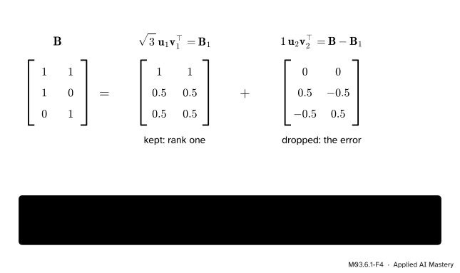
The running rectangular matrix.\(\mat{B} = \begin{bmatrix} 1 & 1 \\ 1 & 0 \\ 0 & 1 \end{bmatrix}\) has \(\sigma_1 = \sqrt3\) with \(\vect{u}_1 = {(2, 1, 1)/\sqrt6}\), \(\vect{v}_1 = {(1, 1)/\sqrt2}\), and \(\sigma_2 = 1\) with \(\vect{u}_2 = {(0, 1, -1)/\sqrt2}\), \(\vect{v}_2 = {(1, -1)/\sqrt2}\) (M03.5.3). The first layer is
because \({\sqrt6\,\sqrt2} = \sqrt{12} = 2\sqrt3\). Subtracting it from \(\mat{B}\) leaves the second layer.
M03.6.1-F4
\(\mat{B}\) split into its two layers. The dropped layer is the error, and both of its norms are \(\sigma_2 = 1\).
The error \(\mat{B} - \mat{B}_1\) has four entries of size \(0.5\), so its squared Frobenius norm is \({4 \times 0.25} = 1 = \sigma_2^2\), as Result 2 says. The error matrix has rank one, so its only singular value, \(1\), is its spectral norm, as Result 3 says. \(\mat{B}_1\) keeps \(3/(3 + 1) = 75\%\) of the energy.
A rank-2 matrix plus a small change. Rows 1 and 2 of \(\mat{R} = \begin{bmatrix} 1 & 1 & 0 \\ 1 & 1 & 0 \\ 0 & 0 & 1 \end{bmatrix}\) are equal, so \(\mat{R}\) has rank 2. Suppose it is measured with small errors:
Now \(\det\mat{M} = {1.05^2 - 0.95^2} = 0.2\), so \(\mat{M}\) has full rank. It is symmetric, and one multiplication each checks three perpendicular eigenvectors: \({\mat{M}(1, 1, 0)} = (2, 2, 0)\), \({\mat{M}(0, 0, 1)} = (0, 0, 1)\) and \({\mat{M}(1, -1, 0)} = (0.1, -0.1, 0)\). The eigenvalues \(2\), \(1\) and \(0.1\) are positive, so they are also the singular values (M03.5.4). Dropping the last layer removes \({0.1 \cdot \tfrac12 (1, -1, 0)(1, -1, 0)\T}\), which is exactly the change, so \(\mat{M}_2 = \mat{R}\). Truncation has filtered the noise out, and \(\norm{\mat{M} - \mat{M}_2}_F = \norm{\mat{M} - \mat{M}_2}_2 = 0.1\).
Code
From scratch: the truncation as a sum of outer products, and the two error formulas.
import numpy as npdef truncate(A, k):"""A_k: the sum of the first k layers sigma_i u_i v_i^T.""" U, s, Vt = np.linalg.svd(np.asarray(A, dtype=float), full_matrices=False)returnsum(s[i] * np.outer(U[:, i], Vt[i]) for i inrange(k))B = np.array([[1.0, 1.0], [1.0, 0.0], [0.0, 1.0]])M = np.array([[1.05, 0.95, 0.0], [0.95, 1.05, 0.0], [0.0, 0.0, 1.0]])print("B_1 =\n", truncate(B, 1).round(10))print("singular values of M:", np.linalg.svd(M, compute_uv=False).round(10))print("M_2 =\n", truncate(M, 2).round(10))rng = np.random.default_rng(0)A = rng.normal(size=(6, 5))s = np.linalg.svd(A, compute_uv=False)for k inrange(1, 5): E = A - truncate(A, k)print(k, "Frobenius:", np.isclose(np.linalg.norm(E, "fro") **2, np.sum(s[k:] **2))," spectral:", np.isclose(np.linalg.norm(E, 2), s[k]))
Now the theorem against rivals. A random matrix of rank \(k\) is a product of a \(6 \times k\) and a \(k \times 5\) matrix. We also try small nudges of \(\mat{A}_k\) itself, which stay at rank \(k\).
k =2U, s, Vt = np.linalg.svd(A, full_matrices=False)best_F, best_2 = np.linalg.norm(A - truncate(A, k), "fro"), s[k]worst_gap_F, worst_gap_2 = np.inf, np.inffor trial inrange(20000):if trial %2==0: # a random rank-2 matrix X = rng.normal(size=(6, k)) @ rng.normal(size=(k, 5))else: # a small nudge of the two factors of A_2 left = U[:, :k] * s[:k] +0.05* rng.normal(size=(6, k)) X = left @ (Vt[:k] +0.05* rng.normal(size=(k, 5))) worst_gap_F =min(worst_gap_F, np.linalg.norm(A - X, "fro") - best_F) worst_gap_2 =min(worst_gap_2, np.linalg.norm(A - X, 2) - best_2)print("best errors:", round(best_F, 4), round(best_2, 4))print("every rival farther away, in both norms:", worst_gap_F >0and worst_gap_2 >0)
best errors: 2.11 1.9014
every rival farther away, in both norms: True
Twenty thousand rivals, and every one of them is farther from \(\mat{A}\) in both norms. A test of this kind cannot prove the theorem, but a single counterexample would have disproved it.
Explore
The module’s interactive, the rank slider, is in the next lesson. It rebuilds the \(48 \times 48\) picture of the second figure from its first \(k\) layers, for every \(k\) from 1 to 48, and prints the energy kept, which by Result 2 is the share of the sum of the \(\sigma_i^2\).
Pitfalls
M03.6.1-F5
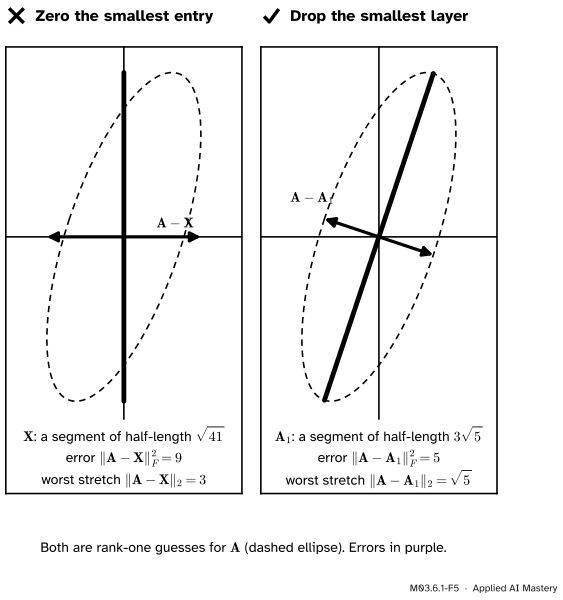
Wrong beside right. Both guesses have rank one. Zeroing the entry 3 of \(\mat{A}\) leaves an error of size 9 in squared Frobenius norm; dropping the small layer leaves only \(\sigma_2^2 = 5\).
“To simplify a matrix, set its smallest entries to zero.”
Small entries are not small layers. For \(\mat{A} = \begin{bmatrix} 3 & 0 \\ 4 & 5 \end{bmatrix}\), zeroing the 3 gives a rank-one matrix \(\mat{X}\) whose error has squared Frobenius norm 9 and spectral norm 3. The truncation \(\mat{A}_1\) gives 5 and \(\sqrt5 \approx 2.24\). Size lives in the singular values, which mix all the entries.
“The error of \(\mat{A}_k\) is \(\sigma_{k+1}\), whatever norm I use.”
Only in the spectral norm. In the Frobenius norm every dropped layer counts. With singular values 5, 4, 3, 2, 1 and \(k = 2\), the spectral error is 3 but the Frobenius error is \(\sqrt{9 + 4 + 1} = \sqrt{14} \approx 3.74\).
“Keeping the largest eigenvalue term does the same job.”
For a symmetric matrix with non-negative eigenvalues it does, because there the two decompositions agree. For the running \(\mat{A} = \begin{bmatrix} 4 & 1 \\ 2 & 3 \end{bmatrix}\) the eigenvalue-5 term of \(\mat{P}\mat{D}\mat{P}^{-1}\) is \(\tfrac53\begin{bmatrix} 2 & 1 \\ 2 & 1 \end{bmatrix}\), and its error has squared Frobenius norm \(40/9 \approx 4.44\). The best rank-one copy does better: \(\sigma_2^2 = 15 - 5\sqrt5 \approx 3.82\). Eigenvectors that are not perpendicular do not give perpendicular layers, and Result 2 needs perpendicular layers.
Check yourself
Recall
1. What is the truncation \(\mat{A}_k\), and what is its rank?
Show answer
The sum of the first \(k\) layers \({\sigma_i\,\vect{u}_i\vect{v}_i\T}\) of the SVD. It has rank \(k\) (when \(k \le r\)).
2. What is \(\norm{\mat{A} - \mat{A}_k}_F^2\)?
Show answer
The sum of the squared singular values that were dropped, \({\sigma_{k+1}^2 + \cdots + \sigma_r^2}\).
3. What is \(\norm{\mat{A} - \mat{A}_k}_2\), and which unit vector is stretched that much?
Show answer
\(\sigma_{k+1}\), the largest dropped singular value. The error stretches \(\vect{v}_{k+1}\) by exactly that much.
4. Why are the layers \({\vect{u}_i\vect{v}_i\T}\) perpendicular to one another?
Show answer
Their entrywise dot product is \({(\vect{u}_i \cdot \vect{u}_j)(\vect{v}_i \cdot \vect{v}_j)}\), which is 0 for \(i \ne j\) and 1 for \(i = j\), because the \(\vect{u}\)’s and the \(\vect{v}\)’s are orthonormal.
5. What does the Eckart-Young theorem say?
Show answer
No matrix of rank at most \(k\) is closer to \(\mat{A}\) than \(\mat{A}_k\), in the spectral norm or in the Frobenius norm.
Exercises
1.★ A matrix has singular values 10, 6, 3 and 1. Find the Frobenius and the spectral error of \(\mat{A}_2\), and the share of the energy it keeps.
Show solution
The dropped values are 3 and 1. The Frobenius error is \(\sqrt{9 + 1} = \sqrt{10} \approx 3.16\) and the spectral error is \(\sigma_3 = 3\). The energy is \(100 + 36 + 9 + 1 = 146\), of which \(\mat{A}_2\) keeps \(136\), a share of \(136/146 \approx 93.2\%\).
2.★★ The running symmetric matrix \(\mat{S} = \begin{bmatrix} 2 & 1 \\ 1 & 2 \end{bmatrix}\) has eigenvalues 3 and 1 with eigenvectors \({(1, 1)/\sqrt2}\) and \({(1, -1)/\sqrt2}\). Find its best rank-one approximation and both errors.
Show solution
The eigenvalues are positive, so they are the singular values and \(\vect{u}_i = \vect{v}_i\). Then
The error \(\mat{S} - \mat{S}_1\) has entries \(0.5\) on the diagonal and \(-0.5\) off it. Its squared Frobenius norm is \({4 \times 0.25} = 1 = \sigma_2^2\), and its spectral norm is \(\sigma_2 = 1\).
3.★★★ Show that \(\norm{\mat{Y}}_2 \le \norm{\mat{Y}}_F\) for every matrix \(\mat{Y}\). Deduce, using only the spectral half of the Eckart-Young theorem, that every matrix \(\mat{X}\) of rank at most \(k\) has \(\norm{\mat{A} - \mat{X}}_F \ge \sigma_{k+1}\).
Show solution
By Result 3 with \(k = 0\), \(\norm{\mat{Y}}_2 = {\sigma_1(\mat{Y})}\), and by Result 2 with \(k = 0\), \(\norm{\mat{Y}}_F^2\) is the sum of all the squared singular values of \(\mat{Y}\), which is at least \(\sigma_1(\mat{Y})^2\). Taking square roots, \(\norm{\mat{Y}}_2 \le \norm{\mat{Y}}_F\).
Now put \(\mat{Y} = \mat{A} - \mat{X}\). The spectral half of the theorem gives \(\norm{\mat{A} - \mat{X}}_2 \ge \sigma_{k+1}\), so \(\norm{\mat{A} - \mat{X}}_F \ge \norm{\mat{A} - \mat{X}}_2 \ge \sigma_{k+1}\). This is weaker than the full Frobenius statement, whose bound is \(\sqrt{\sigma_{k+1}^2 + \sigma_{k+2}^2 + \cdots}\), but it needs no new tool.
Summary card
Keep the biggest layers: nothing of the same rank comes closer.
Eckart-Young. No matrix of rank at most \(k\) does better in either norm.
Sources and next steps
Sources. Each was opened and checked against this lesson on 15 November 2026.
Sheldon Axler, Linear Algebra Done Right, 4th edition (open access), Section 7F. Result 7.88 shows that the norm of a linear map is its largest singular value, and result 7.92, “best approximation by linear map whose range has dimension at most k”, proves that chopping the SVD after \(k\) terms leaves an error of exactly \(s_{k+1}\) and that no map of lower rank does better. The proof in the “deeper” block follows it.
Marc Deisenroth, Aldo Faisal and Cheng Soon Ong, Mathematics for Machine Learning, Section 4.6. Theorem 4.25 (the Eckart-Young theorem) gives the truncation as the best rank-\(k\) approximation in the spectral norm, equation (4.94), with error \(\sigma_{k+1}\), equation (4.95), and sketches the same dimension argument.
David Austin, Understanding Linear Algebra, Using singular value decompositions, subsection “Rank k approximations”: the matrices \(A_k\) built from the first \(k\) singular values approximate \(A\) with increasing accuracy and are, in a sense, the closest of rank \(k\).
NumPy, numpy.linalg.svd: with full_matrices=False the shapes are \((m, K)\) and \((K, n)\) for \(K = \min(m, n)\), the singular values are sorted in descending order, and the rows of Vh are the eigenvectors of \(\mat{A}\T\mat{A}\), that is the right singular vectors.