Any matrix sends the unit circle to an ellipse, and two perpendicular inputs land exactly on its axes. Find them for a 2 by 2 matrix, meet the singular values, and read the matrix as a turn, a stretch along the axes and another turn.
M03.5.1L2 Intermediate25 minIn review (what this means)
The maths and code on this page are checked by automated tests on every change, but an independent reader has not signed it off yet. Spot a mistake or a confusing step? Tell us.
Show that a 2 by 2 matrix has a pair of perpendicular unit inputs whose images are perpendicular, using a sign change and the intermediate value theorem.
Define the singular values and singular vectors by A v = sigma u, and check a claimed pair by multiplication.
Derive that the image of the unit circle is an ellipse with semi-axes sigma_1 and sigma_2 along u_1 and u_2.
Read A = U Sigma V-transpose as a turn, a stretch along the axes and a second turn, and contrast singular vectors with eigenvectors.
The question
A square matrix that is not symmetric can have eigenvectors at an awkward angle, or none at all. Yet every matrix, of any shape, has one picture that never fails: it turns the unit circle into an ellipse. Which inputs land on the axes of that ellipse, how long are the axes, and why is this the single most useful fact about a data matrix?
Intuition
Feed a matrix every unit vector at once: the whole unit circle. M02.4 showed that a matrix keeps a grid a grid, so a round circle cannot come out bent or dented. It comes out as an ellipse, a stretched circle, perhaps squashed flat.
An ellipse has two axes that meet at a right angle: the longest line across it and the shortest. The surprise is on the input side. The two inputs that land on those axes are also perpendicular. Whatever the matrix, there is a right angle going in that is still a right angle coming out.
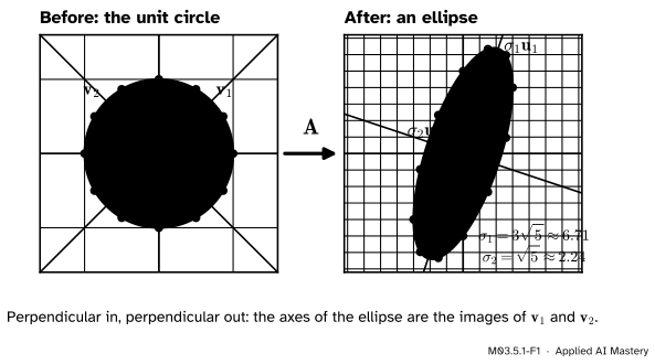
M03.5.1-F1
The running SVD matrix of this course, \(\mat{A} = \begin{bmatrix} 3 & 0 \\ 4 & 5 \end{bmatrix}\), sends the unit circle (left) to an ellipse (right, drawn at a smaller scale). The perpendicular inputs \(\vect{v}_1\) and \(\vect{v}_2\) land on the two axes.
The lengths of the two half-axes are the singular values, \(\sigma_1 \ge \sigma_2\). The input directions are the right singular vectors\(\vect{v}_1, \vect{v}_2\), and the unit vectors along the output axes are the left singular vectors\(\vect{u}_1, \vect{u}_2\). In one line:
\[
\mat{A}\vect{v}_i = \sigma_i\,\vect{u}_i .
\]
That line is the singular value decomposition (SVD), and this module is about it. Machine learning meets it everywhere: compressing an image (M03.6.2), principal component analysis (M03.6.4), least squares (M03.7), the size of a weight matrix (M03.8) and the cheap low-rank updates used to fine-tune large language models.
Build it up
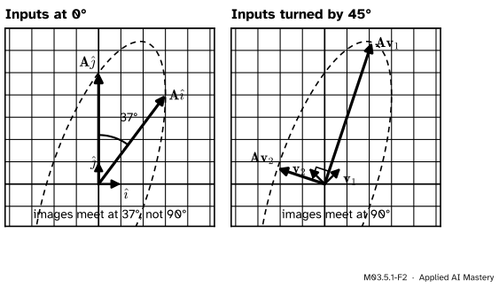
Step 1. Most right angles do not survive. The columns of \(\mat{A}\) are where \(\ihat\) and \(\jhat\) land (M02.4.2): \(\mat{A}\ihat = (3, 4)\) and \(\mat{A}\jhat = (0, 5)\). The inputs are perpendicular, but the outputs are not, because \({(3, 4) \cdot (0, 5)} = 20\), not \(0\). Both have length 5, so the cosine of the angle between them is \(20 / 25 = 0.8\), an angle of about \({37°}\).
Step 2. Turn the input pair. Keep two perpendicular unit inputs and turn them together. Let \(\vect{x}\) point at angle \(\theta\) and let \(\vect{y}\) be \(\vect{x}\) turned by a further \({90°}\):
At \(\theta = 0\) this is the pair \(\ihat, \jhat\) of Step 1. At \(\theta = {45°}\) the images meet at a right angle.
M03.5.1-F2
Turning the perpendicular input pair changes the angle between the two images. At \({0°}\) the images meet at \({37°}\); at \({45°}\) they meet at \({90°}\) and sit on the axes of the ellipse.
Step 3. Measure the angle with one number. The images are perpendicular exactly when the dot product \({\mat{A}\vect{x} \cdot \mat{A}\vect{y}}\) is zero. Write \(c = \cos\theta\) and \(s = \sin\theta\). Then
It is zero when \(2\theta = {90°}\), that is at \(\theta = {45°}\).
The formal statement
The calculation worked for one matrix. A short argument shows that a zero exists for every 2 by 2 matrix, with no calculation at all.
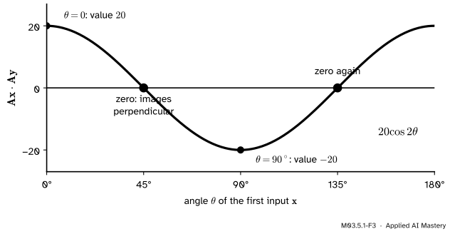
M03.5.1-F3
For the running \(\mat{A}\), the dot product of the two images as the input pair turns. Its value at \({90°}\) is minus its value at \({0°}\), so somewhere between them it must be zero.
Why a zero must exist. Turning the pair by \({90°}\) moves \(\vect{x}\) to where \(\vect{y}\) was, and moves \(\vect{y}\) to \(-\vect{x}\). So the new dot product is
If \(g(0) = 0\) we are done. Otherwise \(g(0)\) and \(g({90°})\) have opposite signs. The function \(g\) is continuous, because it is built from sines and cosines by adding and multiplying, so by the intermediate value theorem (M04.1.4) it is zero at some angle in between. At that angle the two inputs are perpendicular and so are their images.
NoteDefinition: singular values and singular vectors
Let \(\vect{v}_1, \vect{v}_2\) be perpendicular unit inputs whose images are perpendicular, named so that \(\mat{A}\vect{v}_1\) is at least as long as \(\mat{A}\vect{v}_2\). The singular values are the lengths
When \(\sigma_i > 0\), the left singular vector is the unit vector \(\vect{u}_i = \mat{A}\vect{v}_i / \sigma_i\), so that \(\mat{A}\vect{v}_i = \sigma_i\vect{u}_i\). The \(\vect{v}_i\) are the right singular vectors.
The image is an ellipse. Any unit vector is \({\vect{x} = c_1\vect{v}_1 + c_2\vect{v}_2}\) with \({c_1^2 + c_2^2 = 1}\), because the \(\vect{v}_i\) are orthonormal (M02.10.1). By linearity
So the image has coordinates \(y_1 = \sigma_1 c_1\) and \(y_2 = \sigma_2 c_2\) along the perpendicular directions \(\vect{u}_1, \vect{u}_2\). When \(\sigma_2 > 0\), put \(c_i = y_i / \sigma_i\) into \({c_1^2 + c_2^2 = 1}\):
That is an ellipse with half-axes \(\sigma_1\) along \(\vect{u}_1\) and \(\sigma_2\) along \(\vect{u}_2\). If \(\sigma_2 = 0\), the circle is squashed onto a segment of half-length \(\sigma_1\). The same formula shows that \(\norm{\mat{A}\vect{x}}^2 = {\sigma_1^2c_1^2 + \sigma_2^2c_2^2}\) lies between \(\sigma_2^2\) and \(\sigma_1^2\): no unit vector is stretched more than \(\sigma_1\) or less than \(\sigma_2\).
Three matrices. Put the \(\vect{v}_i\) in the columns of \(\mat{V}\), the \(\vect{u}_i\) in the columns of \(\mat{U}\), and the singular values on the diagonal of \(\mat{\Sigma}\). Column \(i\) of \(\mat{A}\mat{V}\) is \(\mat{A}\vect{v}_i\), and column \(i\) of \(\mat{U}\mat{\Sigma}\) is \(\sigma_i\vect{u}_i\). The two agree column by column, so
\[
\mat{A}\mat{V} = \mat{U}\mat{\Sigma}.
\]
\(\mat{V}\) has orthonormal columns, so it is an orthogonal matrix and \(\mat{V}^{-1} = \mat{V}\T\) (M02.10.2). Multiplying both sides on the right by \(\mat{V}\T\) gives
NoteThe singular value decomposition of a 2 by 2 matrix
\[
\mat{A} = \mat{U}\,\mat{\Sigma}\,\mat{V}\T
\]
with \(\mat{U}\) and \(\mat{V}\) orthogonal and \(\mat{\Sigma}\) diagonal with entries \(\sigma_1 \ge \sigma_2 \ge 0\). (If \(\sigma_2 = 0\), take \(\vect{u}_2\) to be either unit vector perpendicular to \(\vect{u}_1\).)
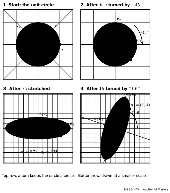
Read it right to left. Applied to \(\vect{x}\), \(\mat{V}\T\vect{x}\) lists the coordinates \({(\vect{v}_1 \cdot \vect{x},\; \vect{v}_2 \cdot \vect{x})}\), which turns the plane so that \(\vect{v}_1, \vect{v}_2\) lie on the axes. Then \(\mat{\Sigma}\) stretches along the axes by \(\sigma_1\) and \(\sigma_2\). Then \(\mat{U}\) turns the axes onto \(\vect{u}_1, \vect{u}_2\). Every matrix is a turn, a stretch, and a turn. “Turn” here means an orthogonal matrix, so it may be a turn-over (a reflection) rather than a rotation.
M03.5.1-F5
The signature picture of the SVD: turn, stretch, turn. The black dot follows the tip of \(\ihat\) and ends at the first column of \(\mat{A}\), \((3, 4)\).
Worked example
Check that \(\vect{v}_1 = (1, 1)/\sqrt{2}\) and \(\vect{v}_2 = (-1, 1)/\sqrt{2}\) are the right singular vectors of \(\mat{A} = \begin{bmatrix} 3 & 0 \\ 4 & 5 \end{bmatrix}\), and find the rest.
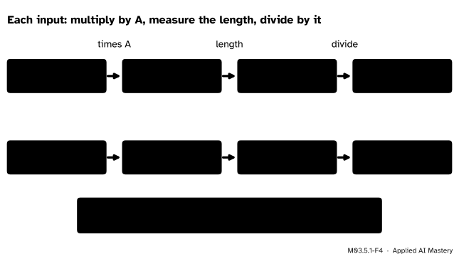
They are perpendicular unit vectors: \({\vect{v}_1 \cdot \vect{v}_2} = (-1 + 1)/2 = 0\), and each has length \(\sqrt{2}/\sqrt{2} = 1\). Multiply each by \(\mat{A}\):
The worked example as a trace: multiply by \(\mat{A}\), measure the length, divide by it.
Read off the turns.\(\mat{V} = \tfrac{1}{\sqrt{2}}\begin{bmatrix} 1 & -1 \\ 1 & 1 \end{bmatrix}\) is the rotation by \({45°}\), so \(\mat{V}\T\) turns by \(-{45°}\). \(\mat{U} = \tfrac{1}{\sqrt{10}}\begin{bmatrix} 1 & -3 \\ 3 & 1 \end{bmatrix}\) is a rotation too (determinant \({(1 + 9)/10} = 1\)), by the angle whose tangent is \(3\), about \({71.57°}\).
Two cross-checks. The area factor of \(\mat{A}\) is \(\det\mat{A} = {3 \cdot 5 - 0 \cdot 4} = 15\) (M02.8.1), and the turns change no area, so it must equal \({\sigma_1\sigma_2}\). It does: \({3\sqrt{5} \cdot \sqrt{5}} = 15\). And the eigenvalues of this triangular matrix are its diagonal entries, \(3\) and \(5\) (M03.1). They are not the singular values: no eigenvector stretches by \(6.708\), the most any input is stretched.
Code
First from scratch: find the angle where the two images become perpendicular by halving an interval on which \(g\) changes sign (bisection), then measure and divide.
import numpy as npA = np.array([[3.0, 0.0], [4.0, 5.0]])def g(theta):"""Dot product of the images of x at angle theta and of x turned by 90 degrees.""" x = np.array([np.cos(theta), np.sin(theta)]) y = np.array([-np.sin(theta), np.cos(theta)])return (A @ x) @ (A @ y)lo, hi =0.0, np.pi /2# g(90 degrees) = -g(0): a sign changeprint("g(0) =", round(g(lo), 9), " g(90) =", round(g(hi), 9))for _ inrange(60): # bisection: keep the half where the sign changes mid = (lo + hi) /2if np.sign(g(mid)) == np.sign(g(lo)): lo = midelse: hi = midtheta = (lo + hi) /2v1 = np.array([np.cos(theta), np.sin(theta)])v2 = np.array([-np.sin(theta), np.cos(theta)])s1, s2 = np.linalg.norm(A @ v1), np.linalg.norm(A @ v2)if s1 < s2: # name them so that sigma_1 is the larger v1, v2, s1, s2 = v2, v1, s2, s1u1, u2 = A @ v1 / s1, A @ v2 / s2print("angle:", round(np.degrees(theta), 6), "degrees")print("sigma:", round(s1, 6), round(s2, 6))print("u1 * sqrt(10):", np.round(u1 * np.sqrt(10), 6), " u2 * sqrt(10):", np.round(u2 * np.sqrt(10), 6))
Assemble the three matrices and multiply them back together, then compare with the eigenvalues.
U = np.column_stack([u1, u2])Sigma = np.diag([s1, s2])V = np.column_stack([v1, v2])print("U Sigma V^T =\n", np.round(U @ Sigma @ V.T, 12))print("det U, det V:", round(np.linalg.det(U), 9), round(np.linalg.det(V), 9))print("turn of U:", round(np.degrees(np.arctan2(U[1, 0], U[0, 0])), 2), "degrees")print("eigenvalues of A:", np.sort(np.linalg.eigvals(A).real))
U Sigma V^T =
 [[3. 0.]
 [4. 5.]]
det U, det V: 1.0 1.0
turn of U: 71.57 degrees
eigenvalues of A: [3. 5.]
The library does all of this in one call. NumPy returns \(\mat{V}\T\) itself, under the name Vh.
U_np, s_np, Vh = np.linalg.svd(A)print("singular values:", s_np)print("first row of Vh:", Vh[0], " first column of U:", U_np[:, 0])
singular values: [6.70820393 2.23606798]
first row of Vh: [-0.70710678 -0.70710678]   first column of U: [-0.31622777 -0.9486833 ]
The singular values agree. The vectors may come back with the opposite sign: flipping both \(\vect{v}_i\) and \(\vect{u}_i\) keeps \({\mat{A}\vect{v}_i = \sigma_i\vect{u}_i}\) true. The next lesson returns to that.
Explore
M03.5-X1
Rotate, stretch, rotate
Choose a matrix with the sliders or by dragging the images of \(\ihat\) and \(\jhat\), then press the step buttons to apply \(\mat{V}\T\), \(\mat{\Sigma}\) and \(\mat{U}\) one at a time. Compare the singular values with the eigenvalues: try the symmetric preset, the shear and the rotation.
Pitfalls
M03.5.1-F6
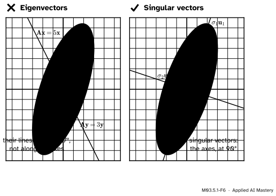
Wrong beside right. The eigenvectors of \(\mat{A}\) stay on their own lines, but those lines are not the axes of the ellipse. The singular vectors land on the axes.
“The axes of the ellipse point along the eigenvectors.”
They do for a symmetric matrix, but not in general. Here the eigenvectors are \((0, 1)\), stretched by \(5\), and \((1, -2)\), stretched by \(3\). Their lines cross at about \({27°}\), and neither runs along an axis of the ellipse. An eigenvector asks “which input keeps its direction?”; a singular vector asks “which perpendicular inputs stay perpendicular?”. The questions are different, and so are the answers.
“The singular values are the eigenvalues, without their signs.”
For \(\mat{A}\) the eigenvalues are \(5\) and \(3\), and the singular values are about \(6.708\) and \(2.236\). Only special matrices make them agree (lesson M03.5.4 shows when). What does survive is the product: both pairs multiply to \(\abs{\det\mat{A}} = 15\).
“\(\mat{U}\) and \(\mat{V}\) are always rotations.”
They are orthogonal, so each is a rotation or a reflection. Taking determinants of \(\mat{A} = \mat{U}\mat{\Sigma}\mat{V}\T\) gives \(\det\mat{A} = {\det\mat{U} \cdot \sigma_1\sigma_2 \cdot \det\mat{V}}\), with each of \(\det\mat{U}\) and \(\det\mat{V}\) equal to \(\pm 1\). A matrix with a negative determinant turns the plane over, so one of the two must be a reflection.
Check yourself
Recall
1. What does every 2 by 2 matrix do to the unit circle?
Show answer
It sends it to an ellipse, or to a segment or a point when the matrix squashes the plane. The half-axes have lengths \(\sigma_1\) and \(\sigma_2\).
2. State the equation that links a right singular vector, a singular value and a left singular vector.
Show answer
\(\mat{A}\vect{v}_i = \sigma_i\vect{u}_i\), with \(\vect{v}_i\) and \(\vect{u}_i\) unit vectors and \(\sigma_i \ge 0\).
3. In \(\mat{A} = \mat{U}\mat{\Sigma}\mat{V}\T\), what does each factor do to the plane?
Show answer
\(\mat{V}\T\) turns the \(\vect{v}_i\) onto the axes, \(\mat{\Sigma}\) stretches along the axes by the singular values, and \(\mat{U}\) turns the axes onto the \(\vect{u}_i\). “Turn” may mean a reflection.
4. Why must the dot product of the two images change sign as the perpendicular input pair turns through \({90°}\)?
Show answer
Turning by \({90°}\) sends \((\vect{x}, \vect{y})\) to \((\vect{y}, -\vect{x})\), so the dot product \({\mat{A}\vect{x} \cdot \mat{A}\vect{y}}\) becomes its own negative.
5. What are the singular values of \(\begin{bmatrix} 3 & 0 \\ 4 & 5 \end{bmatrix}\), and how does their product compare with the determinant?
Show answer
\(\sigma_1 = 3\sqrt{5} \approx 6.708\) and \(\sigma_2 = \sqrt{5} \approx 2.236\). Their product is \(15 = \det\mat{A}\).
Exercises
1.★ Find the singular values and singular vectors of \(\mat{M} = \begin{bmatrix} 2 & 0 \\ 0 & -3 \end{bmatrix}\), and describe the ellipse.
Show solution
The inputs \(\jhat\) and \(\ihat\) are perpendicular and so are their images, \(\mat{M}\jhat = (0, -3)\) and \(\mat{M}\ihat = (2, 0)\). The longer image comes from \(\jhat\), so \(\vect{v}_1 = (0, 1)\), \(\sigma_1 = 3\), \(\vect{u}_1 = (0, -1)\), and \(\vect{v}_2 = (1, 0)\), \(\sigma_2 = 2\), \(\vect{u}_2 = (1, 0)\). The ellipse has half-axis \(3\) upright and \(2\) across. The minus sign is not a singular value: it went into \(\vect{u}_1\).
2.★★ For the shear \(\mat{H} = \begin{bmatrix} 1 & 1 \\ 0 & 1 \end{bmatrix}\), find \({g(\theta) = \mat{H}\vect{x} \cdot \mat{H}\vect{y}}\) with \(\vect{x}\) and \(\vect{y}\) as in the lesson. Find the angle where it is zero, and the singular values.
Show solution
\(\mat{H}\vect{x} = (c + s,\; s)\) and \(\mat{H}\vect{y} = (c - s,\; c)\). So
It is zero when \(\tan 2\theta = -2\). Between \({0°}\) and \({90°}\) that gives \(2\theta \approx {116.57°}\), so \(\theta \approx {58.28°}\) and \(\vect{v}_1 \approx (0.526, 0.851)\). Then \(\mat{H}\vect{v}_1 \approx (1.376, 0.851)\), of length \(\sigma_1 \approx 1.618\). The other input, \(\vect{v}_2 \approx (-0.851, 0.526)\), gives \(\mat{H}\vect{v}_2 \approx (-0.325, 0.526)\), of length \(\sigma_2 \approx 0.618\). These are the golden ratio \({(1 + \sqrt{5})/2}\) and its reciprocal, and their product is \(1 = \det\mat{H}\).
3.★★★ Prove that for every 2 by 2 matrix, \({\sigma_1\sigma_2} = \abs{\det\mat{A}}\), and explain the result as a statement about areas.
Show solution
The determinant of a product is the product of the determinants (M02.8.3), so
\(\mat{U}\) and \(\mat{V}\) are orthogonal, so their determinants are \(\pm 1\) (M02.10.2), and \(\det\mat{V}\T = \det\mat{V}\). \(\mat{\Sigma}\) is diagonal, so \(\det\mat{\Sigma} = \sigma_1\sigma_2\). Taking absolute values, \(\abs{\det\mat{A}} = \sigma_1\sigma_2\). As areas: the unit disc has area \(\pi\) and the ellipse has area \({\pi\sigma_1\sigma_2}\), so the map multiplies areas by \({\sigma_1\sigma_2}\), which is what \(\abs{\det\mat{A}}\) measures. The turns change no area; only the stretch does.
Summary card
Every matrix sends perpendicular inputs \(\vect{v}_1, \vect{v}_2\) to perpendicular outputs along the axes of an ellipse.
M03.5.1-F1
A circle in, an ellipse out.
Singular triplets.\(\mat{A}\vect{v}_i = \sigma_i\vect{u}_i\), with \(\sigma_1 \ge \sigma_2 \ge 0\).
Ellipse. Half-axes \(\sigma_1\) along \(\vect{u}_1\) and \(\sigma_2\) along \(\vect{u}_2\).
Not eigenvalues. Eigenvalues \(5\) and \(3\); only \(\abs{\det\mat{A}} = 15\) is shared.
Sources and next steps
Sources. Each was opened and checked against this lesson on 15 November 2026.
David Austin, Understanding Linear Algebra, section “Singular value decompositions”. The unit circle mapped to an ellipse, the relation \(\mat{A}\vect{v}_i = \sigma_i\vect{u}_i\) and singular values listed in decreasing order.
Marc Peter Deisenroth, A. Aldo Faisal and Cheng Soon Ong, Mathematics for Machine Learning, Section 4.5: Theorem 4.22 (the SVD theorem) and Figure 4.8, which reads the SVD as a basis change by \(\mat{V}\T\), a scaling by \(\mat{\Sigma}\) and a basis change by \(\mat{U}\).
Sheldon Axler, Linear Algebra Done Right, 4th edition, Section 7E: the table after 7.68 comparing eigenvalues with singular values (singular values are non-negative and always listed in decreasing order).
Gilbert Strang, Singular value decomposition, MIT OpenCourseWare 18.06SC, lecture 29: \(\mat{A} = \mat{U}\mat{\Sigma}\mat{V}\T\) with \(\mat{U}\) and \(\mat{V}\) orthogonal.
NumPy reference, numpy.linalg.svd: returns U, S and Vh, with the singular values sorted in descending order.