Every positive definite matrix factors as L times L-transpose with L lower triangular. Derive the entries one by one, see that the method works exactly when the matrix is positive definite, and use it to solve systems and to draw correlated Gaussian samples.
M03.4.3L2 Intermediate25 minIn review (what this means)
The maths and code on this page are checked by automated tests on every change, but an independent reader has not signed it off yet. Spot a mistake or a confusing step? Tell us.
Derive the Cholesky factor of a 2 by 2 and a 3 by 3 positive definite matrix entry by entry, and state the general algorithm.
Explain why the algorithm succeeds exactly when the matrix is positive definite, and use it as a test.
Solve S x = b with one forward and one back substitution once S = L L-transpose is known.
Draw samples with a given covariance C as mu + L z from independent standard samples z, and prove that their covariance is L L-transpose.
The question
A simulation needs pairs of numbers that rise and fall together, with variances 4 and 3 and covariance 2, but a random number generator only gives independent numbers with variance 1. A Gaussian process needs to solve the same large symmetric system again and again. Both jobs call for a square root of a positive definite matrix. Which square root, and how is it found?
From the last lesson
1. What is the quick test for a symmetric 2 by 2 matrix to be positive definite?
Show answer
\({a > 0}\) and \({ac - b^2 > 0}\).
2. Why is \({\mat{X}\T\mat{X}}\) always positive semidefinite?
Show answer
Because \({\vect{w}\T\mat{X}\T\mat{X}\vect{w} = \norm{\mat{X}\vect{w}}^2 \geq 0}\).
Intuition
A positive number has a square root: \({9 = 3 \times 3}\). A positive definite matrix has one too, and the most useful one is made of triangles.
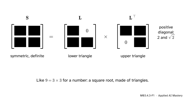
M03.4.3-F1
The Cholesky factorisation of the matrix with rows \({(4, 2)}\) and \({(2, 3)}\). The factor \(\mat{L}\) is lower triangular with a positive diagonal, and the matrix is \(\mat{L}\) times its own transpose.
Why call it a square root? Because the form becomes a length squared:
That is the Gram matrix of the last lesson with \({\mat{X} = \mat{L}\T}\). And the triangles are what make it cheap: a triangular system is solved one unknown at a time.
Build it up
Step 1. Multiply out a triangle times its transpose. Write \(\mat{L} = \begin{bmatrix} l_{11} & 0 \\ l_{21} & l_{22} \end{bmatrix}\). Row times column:
Step 2. Match the entries in order. Set this equal to \(\begin{bmatrix} a & b \\ b & c \end{bmatrix}\) and read off one unknown at a time:
\[
\begin{aligned}
l_{11}^2 = a \;&\Rightarrow\; l_{11} = \sqrt{a}, \\
l_{11}l_{21} = b \;&\Rightarrow\; l_{21} = b / l_{11}, \\
l_{21}^2 + l_{22}^2 = c \;&\Rightarrow\; l_{22} = \sqrt{c - l_{21}^2} .
\end{aligned}
\]
Step 3. See when it works. The first root needs \({a > 0}\). The second needs
\[
\begin{aligned}
c - l_{21}^2 &= c - \frac{b^2}{a} \\
&= \frac{ac - b^2}{a} > 0 .
\end{aligned}
\]
Those are exactly the two pivots of the last lesson. So the method runs to the end exactly when \({a > 0}\) and \({ac - b^2 > 0}\): when the matrix is positive definite. Each diagonal entry of \(\mat{L}\) is the square root of a pivot.
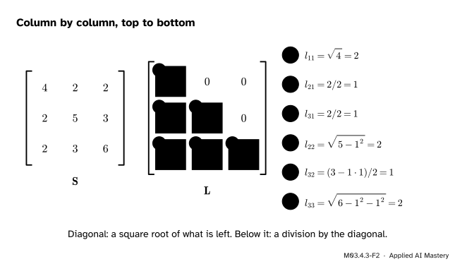
Step 4. Three by three. The same matching works column by column. Each diagonal entry is the square root of what is left of \(s_{jj}\) after the squares already used; each entry below it is what is left of \(s_{ij}\), divided by the diagonal entry.
M03.4.3-F2
The order of the computation on a 3 by 3 example. Every entry needs only entries found before it.
The formal statement
NoteTheorem: Cholesky factorisation
A symmetric matrix \(\mat{S}\) is positive definite if and only if it can be written as \({\mat{S} = \mat{L}\mat{L}\T}\) with \(\mat{L}\) lower triangular and every diagonal entry of \(\mat{L}\) positive. The factor \(\mat{L}\) is then unique. Its entries are found column by column, for \({j = 1, \dots, n}\):
Why the formulas. Entry \({(i, j)}\) of \({\mat{L}\mat{L}\T}\) is row \(i\) of \(\mat{L}\) dotted with row \(j\) of \(\mat{L}\), that is, the sum of \(l_{ik}l_{jk}\) over \(k\). Row \(j\) stops at \({k = j}\), so for \(i \geq j\) the sum runs to \({k = j}\). Its last term is \(l_{ij}l_{jj}\); the earlier terms use columns already found. Solving for that last term gives the two formulas, the first with \({i = j}\).
If \({\mat{S} = \mat{L}\mat{L}\T}\) then \(\mat{S}\) is positive definite. We showed \({\vect{x}\T\mat{S}\vect{x} = \norm{\mat{L}\T\vect{x}}^2 \geq 0}\). A triangular matrix with a positive diagonal has determinant equal to the product of the diagonal, which is not zero, so \({\mat{L}\T\vect{x} = \vect{0}}\) only for \({\vect{x} = \vect{0}}\).
If \(\mat{S}\) is positive definite, every square root is of a positive number. The number under the \(j\)-th root is the \(j\)-th pivot of elimination on \(\mat{S}\): dividing row \(j\) of elimination by the square root of its pivot is exactly what produces row \(j\) of \(\mat{L}\T\). By the pivot test of the last lesson, every pivot of a positive definite matrix is positive. Uniqueness holds because each formula leaves no choice once the diagonal is required to be positive.
A test that costs half of elimination. Entry \({(i, j)}\) costs \({j - 1}\) multiply-and-add updates, and adding these over the lower triangle gives about \(n^3/6\), against about \(n^3/3\) for elimination (M02.6.4): symmetry lets Cholesky do half the work. If some number under a root is zero or negative, the matrix is not positive definite, and the method has found that out without computing a single eigenvalue.
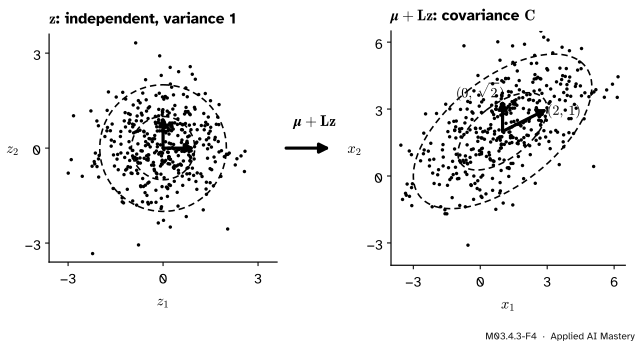
Correlated samples. Let \(\vect{z}\) have independent entries with mean 0 and variance 1, so that its covariance matrix is \({\E[\vect{z}\vect{z}\T] = \mat{I}}\). Put \({\vect{x} = \vect{\mu} + \mat{L}\vect{z}}\). Then \({\vect{x} - \vect{\mu} = \mat{L}\vect{z}}\), and by linearity of expectation
If \(\vect{z}\) is Gaussian, so is \(\vect{x}\): this is a standard way to sample a multivariate Gaussian (M07.3), and the same linear move of a random variable is used to compute gradients when training variational autoencoders.
M03.4.3-F4
Independent samples (left) become correlated ones (right). The unit arrows go to the columns of \(\mat{L}\), and the dashed circles become the ellipses of the target covariance.
Worked example
Factor. For \(\mat{S}\) with rows \({(4, 2)}\) and \({(2, 3)}\): \({l_{11} = \sqrt4 = 2}\), then \({l_{21} = 2/2 = 1}\), then \({l_{22} = \sqrt{3 - 1^2} = \sqrt2}\). Check:
The squares of the diagonal, 4 and 2, are the pivots, and their product 8 is \(\det\mat{S}\).
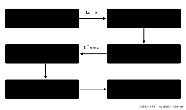
Solve \({\mat{S}\vect{x} = \vect{b}}\) with \({\vect{b} = (6, 5)}\). Write \({\mat{L}\mat{L}\T\vect{x} = \vect{b}}\) as two triangular systems, with \({\vect{z} = \mat{L}\T\vect{x}}\) in between. Forward through \({\mat{L}\vect{z} = \vect{b}}\), top row first:
So \({\vect{x} = (1, 1)}\), and indeed \({\mat{S}\vect{x} = (4 + 2,\; 2 + 3)} = (6, 5)\).
M03.4.3-F3
The worked solve as a trace: forward substitution through \(\mat{L}\), then back substitution through \(\mat{L}\T\).
Code
From scratch, straight from the formulas, then the library calls.
import numpy as npdef cholesky(S):"""Lower-triangular L with L L^T = S. Raises ValueError if S is not positive definite.""" S = np.asarray(S, dtype=float) n =len(S) L = np.zeros((n, n))for j inrange(n): left = S[j, j] - L[j, :j] @ L[j, :j]if left <=0:raiseValueError(f"not positive definite: pivot {j +1} is {left:.3g}") L[j, j] = np.sqrt(left)for i inrange(j +1, n): L[i, j] = (S[i, j] - L[i, :j] @ L[j, :j]) / L[j, j]return Ldef forward(L, b): # solve L z = b, top row first z = np.zeros(len(b))for i inrange(len(b)): z[i] = (b[i] - L[i, :i] @ z[:i]) / L[i, i]return zdef back(U, z): # solve U x = z, bottom row first n =len(z) x = np.zeros(n)for i inreversed(range(n)): x[i] = (z[i] - U[i, i +1:] @ x[i +1:]) / U[i, i]return xS = np.array([[4.0, 2.0], [2.0, 3.0]])L = cholesky(S)b = np.array([6.0, 5.0])z = forward(L, b)x = back(L.T, z)print("L =\n", L.round(6), "\nz =", z.round(6), " x =", x.round(6))print("3 by 3:\n", cholesky([[4, 2, 2], [2, 5, 3], [2, 3, 6]]))for name, M in [("saddle", [[1, 2], [2, 1]]), ("trough", [[1, 2], [2, 4]])]:try: cholesky(M)exceptValueErroras err:print(name, "->", err)
L =
 [[2.       0.      ]
 [1.       1.414214]]
z = [3.       1.414214]   x = [1. 1.]
3 by 3:
 [[2. 0. 0.]
 [1. 2. 0.]
 [1. 1. 2.]]
saddle -> not positive definite: pivot 2 is -3
trough -> not positive definite: pivot 2 is 0
The saddle fails at the second pivot, \({-3}\), and the trough at a second pivot of exactly 0. NumPy’s numpy.linalg.cholesky returns the lower factor and raises LinAlgError when the factorisation fails. SciPy splits the job in two: cho_factor factors once, and cho_solve reuses the factor for every new right-hand side.
from scipy.linalg import cho_factor, cho_solveprint("numpy:\n", np.linalg.cholesky(S))try: np.linalg.cholesky(np.array([[1.0, 2.0], [2.0, 1.0]]))except np.linalg.LinAlgError:print("numpy refuses the saddle")factor = cho_factor(S) # (matrix, lower flag); upper triangle by defaultprint("cho_solve:", cho_solve(factor, b), " lower flag:", factor[1])# Correlated samples: mean (1, 2), covariance S.rng = np.random.default_rng(0)Z = rng.normal(size=(200_000, 2))X = np.array([1.0, 2.0]) + Z @ L.T # each row is mu + L zprint("sample mean:", X.mean(axis=0).round(3))print("sample covariance:\n", np.cov(X, rowvar=False).round(3))def updates(n):"""Multiply-and-add updates of Cholesky: entry (i, j) of L costs j - 1 of them (j counted from 1)."""returnsum(j * (n - j) for j inrange(n)) # column j (from 0) has n - j entries, each costing jprint("updates for n = 300:", updates(300), " n^3/6 =", 300**3//6)
The sample covariance comes out close to \(\mat{S}\), within sampling noise, and the count of updates for \({n = 300}\) is within one per cent of \(n^3/6\).
Explore
This module’s interactive, bowl or saddle, lives in lesson M03.4.2. Set the sliders to \({a = 4}\), \({b = 2}\), \({c = 3}\): the read-out shows \({a = 4}\) and \({ac - b^2 = 8}\). They give the pivots 4 and \({8/4 = 2}\), the squares of the diagonal of \(\mat{L}\). Then raise \(b\) until the ellipses open into hyperbolas: that is where Cholesky would stop.
Pitfalls
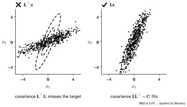
M03.4.3-F5
Wrong beside right, for \(\mat{C}\) with rows \({(1, 2)}\) and \({(2, 5)}\), whose factor has rows \({(1, 0)}\) and \({(2, 1)}\). Multiplying by \(\mat{L}\T\) gives covariance \({\mat{L}\T\mat{L}}\), with rows \({(5, 2)}\) and \({(2, 1)}\): the wrong cloud.
“\(\mat{L}\) or its transpose, it makes no difference.”
It does. The covariance of \({\mat{L}\T\vect{z}}\) is \({\mat{L}\T\mat{L}}\), which is usually a different matrix. In the figure, \(\mat{C}\) has variance 5 along \(x_2\), but \({\mat{L}\T\mat{L}}\) has it along \(x_1\). With samples stored as rows, as in the code, the product is Z @ L.T, which applies \(\mat{L}\) to each row.
“cho_factor returns \(\mat{L}\).”
By default it returns the upper factor \(\mat{L}\T\), together with a flag saying which triangle it used, and the SciPy documentation warns that the other triangle may hold arbitrary values. Pass the pair straight to cho_solve; for \(\mat{L}\) itself, use numpy.linalg.cholesky.
“A covariance matrix always has a Cholesky factor.”
A covariance matrix is only guaranteed to be semidefinite. With a duplicated feature or fewer samples than features it is singular, and Cholesky meets a zero pivot, as for the trough above. In floating point that pivot may come out as a tiny positive or negative number instead of exactly 0, so the method may stop or may return a useless factor. A common remedy is to add a tiny multiple of \(\mat{I}\), which lifts every eigenvalue by that amount, as ridge does in the last lesson.
Check yourself
Recall
1. What shape is the Cholesky factor, and what is special about its diagonal?
Show answer
Lower triangular, with every diagonal entry positive.
2. Give the formulas for the 2 by 2 factor of the matrix with rows \({(a, b)}\) and \({(b, c)}\).
3. What are the squares of the diagonal entries of \(\mat{L}\)?
Show answer
The pivots of elimination on \(\mat{S}\).
4. How do you solve \({\mat{S}\vect{x} = \vect{b}}\) once you have \(\mat{L}\)?
Show answer
Solve \({\mat{L}\vect{z} = \vect{b}}\) by forward substitution, then \({\mat{L}\T\vect{x} = \vect{z}}\) by back substitution.
5. Why do the samples \({\vect{\mu} + \mat{L}\vect{z}}\) have covariance \({\mat{L}\mat{L}\T}\)?
Show answer
Because \({\E[\mat{L}\vect{z}\vect{z}\T\mat{L}\T]} = {\mat{L}\,\E[\vect{z}\vect{z}\T]\,\mat{L}\T}\) and \({\E[\vect{z}\vect{z}\T] = \mat{I}}\).
Exercises
1.★ Find the Cholesky factor of the matrix with rows \({(9, 6)}\) and \({(6, 5)}\), and use it to write \({9x^2 + 12xy + 5y^2}\) as a sum of two squares.
Show solution
\({l_{11} = 3}\), \({l_{21} = 6/3 = 2}\), \({l_{22} = \sqrt{5 - 4} = 1}\), so \(\mat{L}\) has rows \({(3, 0)}\) and \({(2, 1)}\). Then \({\mat{L}\T\vect{x} = {(3x + 2y,\; y)}}\), and the form is \({\norm{\mat{L}\T\vect{x}}^2} = {(3x + 2y)^2 + y^2}\).
2.★★ Factor the matrix with rows \({(4, 2, 2)}\), \({(2, 5, 3)}\) and \({(2, 3, 6)}\) by hand. Compare the squares of the diagonal with the pivots found in the last lesson.
Show solution
Column 1: \({l_{11} = 2}\), \({l_{21} = 1}\), \({l_{31} = 1}\). Column 2: \({l_{22} = \sqrt{5 - 1} = 2}\) and \({l_{32} = (3 - 1 \cdot 1)/2 = 1}\). Column 3: \({l_{33} = \sqrt{6 - 1 - 1} = 2}\). So \(\mat{L}\) has rows \({(2, 0, 0)}\), \({(1, 2, 0)}\) and \({(1, 1, 2)}\). The squares of the diagonal are 4, 4 and 4: the pivots found in Exercise 2 of M03.4.2.
3.★★★ Show that \({\det \mat{S} = (l_{11} l_{22} \cdots l_{nn})^2}\) and that \({\ln\det\mat{S} = 2\sum_i \ln l_{ii}}\). Check both on the worked example.
Show solution
The determinant of a product is the product of the determinants, and transposing does not change a determinant, so \({\det\mat{S} = \det\mat{L}\,\det\mat{L}\T = (\det\mat{L})^2}\). A triangular matrix has as determinant the product of its diagonal. Taking logarithms of the square of a product gives twice the sum of the logarithms, each \(l_{ii}\) being positive. For the worked example, \({(2\sqrt2)^2 = 8 = 4 \cdot 3 - 2^2}\), and \({2(\ln 2 + \ln\sqrt2)} = {\ln 4 + \ln 2} = \ln 8\). This is how the log-likelihood of a Gaussian is computed without ever forming a determinant, which could overflow.
Summary card
A positive definite matrix is a lower triangle times its transpose.
Test. The method succeeds exactly when \(\mat{S}\) is positive definite.
Cost. About \(n^3/6\) updates, half of elimination.
Solve.\({\mat{L}\vect{z} = \vect{b}}\), then \({\mat{L}\T\vect{x} = \vect{z}}\).
Sample.\({\vect{\mu} + \mat{L}\vect{z}}\) has covariance \({\mat{L}\mat{L}\T}\).
Sources and next steps
Sources. Each was opened and checked against this lesson on 15 November 2026.
Marc Peter Deisenroth, A. Aldo Faisal and Cheng Soon Ong, Mathematics for Machine Learning, Section 4.3. Theorem 4.18 states that a symmetric positive definite matrix factors as \({\mat{L}\mat{L}\T}\) with a unique lower-triangular \(\mat{L}\) with positive diagonal; Example 4.10 derives the 3 by 3 entries (equations 4.47 and 4.48); the text after it notes the uses for sampling a Gaussian, for the linear transformation of random variables in the variational autoencoder, and for the determinant as the product of the squared diagonal.
NumPy reference, numpy.linalg.cholesky: returns the lower-triangular factor by default and raises LinAlgError if the matrix is not positive definite.
SciPy reference, scipy.linalg.cho_factor and scipy.linalg.cho_solve: cho_factor returns the pair (matrix, lower), upper-triangular by default, with a warning that the unused part may hold arbitrary data; cho_solve takes that pair and returns the solution of \({\mat{A}\vect{x} = \vect{b}}\).
Gilbert Strang, Positive definite matrices and minima, MIT OpenCourseWare 18.06SC, lecture summary: the coefficients of the completed squares are the pivots and the multipliers of elimination.