The Rayleigh quotient x-transpose S x over x-transpose x is a weighted average of the eigenvalues, so it always lies between the smallest and the largest. For a covariance matrix it is the variance along a direction, which makes the top eigenvector the direction of greatest spread: the first step of PCA.
M03.3.4L2 Intermediate25 minIn review (what this means)
The maths and code on this page are checked by automated tests on every change, but an independent reader has not signed it off yet. Spot a mistake or a confusing step? Tell us.
Define the Rayleigh quotient R(x) = x-transpose S x / x-transpose x and explain why it depends only on the direction of x.
Derive that R(x) is a weighted average of the eigenvalues, and conclude that it lies between the smallest and the largest eigenvalue.
Show that u-transpose C u is the variance of centred data along a unit direction u, and identify the direction of largest variance.
Check the bounds numerically by evaluating R on many random directions and comparing with numpy.linalg.eigh.
The question
A cloud of data points is stretched more in some directions than in others. Principal component analysis starts by asking for the single direction in which the cloud is most spread out. There are infinitely many directions to try. How can one eigenvector of the covariance matrix be guaranteed to beat every one of them?
From the last lesson
1. Write a symmetric matrix as a sum of pieces, and say what each piece is.
Show answer
\(\mat{S} = {\sum_i \lambda_i\vect{q}_i\vect{q}_i\T}\), where each \(\vect{q}_i\vect{q}_i\T\) is the projection onto the line of the unit eigenvector \(\vect{q}_i\).
2. How do you compute \({\mat{S}^{-1}}\) from the pieces, and when does it exist?
Show answer
\({\mat{S}^{-1}} = {\sum_i \lambda_i^{-1}\vect{q}_i\vect{q}_i\T}\), which exists when no eigenvalue is 0.
Intuition
For a unit vector \(\vect{x}\), the number \({\vect{x} \cdot (\mat{S}\vect{x})}\) says how far \(\mat{S}\vect{x}\) reaches in the direction of \(\vect{x}\) itself. Divided by \({\vect{x} \cdot \vect{x}}\), so that the length of \(\vect{x}\) does not matter, it is the Rayleigh quotient
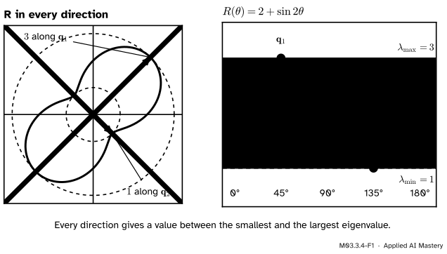
Turn \(\vect{x}\) once round the circle and record \(R\) in every direction.
M03.3.4-F1
The Rayleigh quotient of the running \(\mat{S}\) in every direction. It never leaves the band between the eigenvalues 1 and 3, and it touches the edges exactly at the eigenvectors.
Two things stand out. The values are trapped between the smallest eigenvalue, 1, and the largest, 3. And the extremes are reached exactly at the eigenvectors: the top at \(\vect{q}_1\), the bottom at \(\vect{q}_2\). That is the whole lesson. The rest explains why, and why it answers the question about data.
Build it up
Step 1. Only the direction matters. Replace \(\vect{x}\) by \(s\vect{x}\) for any number \({s \neq 0}\). The top becomes \({s^2\,\vect{x}\T\mat{S}\vect{x}}\) and the bottom \({s^2\,\vect{x}\T\vect{x}}\), and the \(s^2\) cancels. So \(R\) is the same everywhere along a line through the origin, and it is enough to look at unit vectors, for which \({R(\vect{x})} = {\vect{x}\T\mat{S}\vect{x}}\).
For the running \(\mat{S}\) and a unit vector \({(\cos\theta, \sin\theta)}\),
using \({\cos^2\theta + \sin^2\theta} = 1\) and \({2\sin\theta\cos\theta} = {\sin 2\theta}\). A sine swings between \({-1}\) and 1, so \(R\) swings between 1 and 3: the curve in the figure.
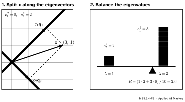
Step 2. In eigen-coordinates, R is an average. Write \(\vect{x} = {c_1\vect{q}_1 + c_2\vect{q}_2}\), with \(c_i = {\vect{q}_i \cdot \vect{x}}\). Then \(\mat{S}\vect{x} = {\lambda_1c_1\vect{q}_1 + \lambda_2c_2\vect{q}_2}\). Dot this with \(\vect{x}\). Because \({\vect{q}_1 \cdot \vect{q}_2} = 0\) and each \(\vect{q}_i\) has length 1, the cross terms vanish:
The two fractions are never negative and add up to 1. \(R\) is a weighted average of the eigenvalues, and each weight is the share of \(\vect{x}\) that lies along that eigenvector.
M03.3.4-F2
The Rayleigh quotient as a balance. Put weight \(c_i^2\) at position \(\lambda_i\); the beam balances at \(R\). For \(\vect{x} = {(3, 1)}\) the weights are 2 and 8, and the balance point is 2.6.
Step 3. An average cannot escape its range. A weighted average of 1 and 3 lies between 1 and 3. It equals 3 only if all the weight sits on 3, that is, only if \(c_2 = 0\) and \(\vect{x}\) lies along \(\vect{q}_1\).
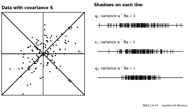
Step 4. For data, R is a variance. Let the rows \({\vect{x}_1, \dots, \vect{x}_n}\) of \(\mat{X}_c\) be centred data points, with covariance matrix \({\mat{C}} = {\mat{X}_c\T\mat{X}_c/(n - 1)} = {\tfrac{1}{n-1}\sum_k \vect{x}_k\vect{x}_k\T}\) (M06.10). Take a unit direction \(\vect{u}\). The shadow of point \(k\) on the line of \(\vect{u}\) has coordinate \({\vect{u} \cdot \vect{x}_k}\); these coordinates have mean 0, because the data are centred. Their sample variance is
The first line writes the square of the number \({\vect{u}\T\vect{x}_k}\) as that number times its transpose \({\vect{x}_k\T\vect{u}}\). So the variance along \(\vect{u}\) is the Rayleigh quotient of the covariance matrix, and by Step 3 the direction of largest variance is the top eigenvector.
M03.3.4-F4
A cloud whose covariance matrix is exactly \(\mat{S}\), and the shadows of its points on three lines. The spread of the shadows is \(\vect{u}\T\mat{S}\vect{u}\): 3 along \(\vect{q}_1\), 2 along the horizontal axis and 1 along \(\vect{q}_2\).
The formal statement
NoteThe Rayleigh quotient theorem
Let \(\mat{S}\) be real symmetric with eigenvalues \(\lambda_{\min} = {\lambda_n \le \cdots \le \lambda_1} = \lambda_{\max}\). For every non-zero \(\vect{x}\),
The upper bound is reached exactly when \(\vect{x}\) is an eigenvector for \(\lambda_{\max}\), and the lower bound exactly when \(\vect{x}\) is an eigenvector for \(\lambda_{\min}\).
Proof. By the spectral theorem, \(\mat{S}\) has orthonormal eigenvectors \({\vect{q}_1, \dots, \vect{q}_n}\), and they form a basis. Write \(\vect{x} = {\sum_i c_i\vect{q}_i}\) with \(c_i = {\vect{q}_i \cdot \vect{x}}\). Then \(\mat{S}\vect{x} = {\sum_i \lambda_ic_i\vect{q}_i}\), and
because \({\vect{q}_j \cdot \vect{q}_i}\) is 1 when \(i = j\) and 0 otherwise. The same step with \(\mat{S} = \mat{I}\) gives \({\vect{x}\T\vect{x}} = {\sum_i c_i^2}\), which is positive because \({\vect{x} \neq \vect{0}}\). Each \(\lambda_i\) is at most \(\lambda_{\max}\), and each \({c_i^2 \ge 0}\), so
Dividing by \({\vect{x}\T\vect{x}}\) gives \({R(\vect{x}) \le \lambda_{\max}}\). The sum is zero exactly when \(c_i = 0\) for every \(i\) with \({\lambda_i < \lambda_{\max}}\), that is, when \(\vect{x}\) is a combination of eigenvectors for \(\lambda_{\max}\), which is an eigenvector for \(\lambda_{\max}\). The lower bound is the same argument with \({{\lambda_i - \lambda_{\min}} \ge 0}\). \(\blacksquare\)
What it means for data. Apply the theorem to a covariance matrix \(\mat{C}\). Over all unit directions, the variance \({\vect{u}\T\mat{C}\vect{u}}\) is largest along the top eigenvector, and the largest variance is the top eigenvalue. That direction is the first principal component, which module M03.6 builds into a full method. The quotient also appeared in lesson M03.2.4 as the power method’s estimate of an eigenvalue. For a symmetric matrix, by this theorem, that estimate can never overshoot \(\lambda_{\max}\). Without symmetry it can: for the running \(\mat{A}\), lesson M03.2.4 found \({R(18, 14)} \approx 5.077\), above the largest eigenvalue 5.
Go deeper: the second direction, and the Courant-Fischer min-max theorem
After the top direction, PCA asks for the direction of largest variance perpendicular to it. If \({\vect{x} \cdot \vect{q}_1} = 0\), then \(c_1 = 0\), and the weighted average runs over \({\lambda_2, \dots, \lambda_n}\) only. So the largest value of \(R\) on the vectors perpendicular to \(\vect{q}_1\) is \(\lambda_2\), reached at \(\vect{q}_2\), and so on down the list.
The Courant-Fischer theorem describes every eigenvalue without naming the earlier eigenvectors. With the eigenvalues in decreasing order,
At least \(\lambda_k\): take \(V\) spanned by \({\vect{q}_1, \dots, \vect{q}_k}\). Every non-zero \(\vect{x}\) in it puts all its weight on \({\lambda_1, \dots, \lambda_k}\), all of which are at least \(\lambda_k\), so \({R(\vect{x}) \ge \lambda_k}\) throughout \(V\).
At most \(\lambda_k\): let \(V\) be any subspace of dimension \(k\), and let \(W\) be spanned by \({\vect{q}_k, \dots, \vect{q}_n}\), of dimension \({n - k + 1}\). The two dimensions add to \({n + 1}\), more than \(n\), so \(V\) and \(W\) share a non-zero vector \(\vect{x}\) (if they shared only \(\vect{0}\), a basis of \(V\) together with a basis of \(W\) would be \({n + 1}\) independent vectors in \(\R^n\)). That \(\vect{x}\) puts all its weight on \({\lambda_k, \dots, \lambda_n}\), so \({R(\vect{x}) \le \lambda_k}\), and the minimum over \(V\) is at most \(\lambda_k\).
Worked example
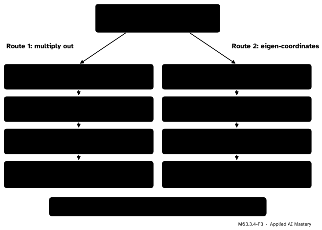
Evaluate \(R\) for \(\mat{S} = \begin{bmatrix} 2 & 1 \\ 1 & 2 \end{bmatrix}\) in four directions, and compute \({R(3, 1)}\) two ways.
Four directions. With \({\vect{x}\T\mat{S}\vect{x}} = {2x^2 + 2xy + 2y^2}\):
\({(1, 0)}\): \({{2}/{1}} = 2\), the top-left entry of \(\mat{S}\).
Route 2, weights.\(c_1 = {\vect{q}_1 \cdot (3, 1)} = {4/\sqrt2}\) and \(c_2 = {\vect{q}_2 \cdot (3, 1)} = {2/\sqrt2}\), so \(c_1^2 = 8\) and \(c_2^2 = 2\), adding to 10 as they must. Then \(R = {3 \cdot \tfrac{8}{10} + 1 \cdot \tfrac{2}{10}} = {2.4 + 0.2} = 2.6\).
A covariance matrix. Lesson M06.10.2 found the covariance matrix \(\mat{C} = \begin{bmatrix} 1/2 & 1/4 \\ 1/4 & 1/2 \end{bmatrix} = \mat{S}/4\), with eigenvalues \({\tfrac34}\) and \({\tfrac14}\). Along the axis \({(1, 0)}\) the variance is \({\tfrac12}\), the variance of the first variable. Along \(\vect{u} = {(1, 1)/\sqrt2}\) it is \({\tfrac12\,(\tfrac12 + \tfrac14 + \tfrac14 + \tfrac12)} = {\tfrac34}\), the largest possible: no weighted combination \({aX + bY}\) with \({a^2 + b^2} = 1\) varies more.
Code
From scratch: throw many random directions at \(R\) and see where the values land.
import numpy as npdef rayleigh(S, x):return (x @ S @ x) / (x @ x)rng = np.random.default_rng(0)S = np.array([[2.0, 1.0], [1.0, 2.0]])S3 = np.array([[2.0, 1.0, 1.0], [1.0, 2.0, 1.0], [1.0, 1.0, 2.0]])for name, M in [("S", S), ("S3", S3)]: xs = rng.normal(size=(20_000, len(M))) # random directions, any lengths values = np.array([rayleigh(M, x) for x in xs])print(f"{name}: R ranges over [{values.min():.4f}, {values.max():.4f}];"f" eigh says [{np.linalg.eigvalsh(M)[0]:.4f}, {np.linalg.eigvalsh(M)[-1]:.4f}]")print("R(3, 1) =", rayleigh(S, np.array([3.0, 1.0])), " R(0, 5) =", rayleigh(S, np.array([0.0, 5.0])))
S: R ranges over [1.0000, 3.0000];  eigh says [1.0000, 3.0000]
S3: R ranges over [1.0000, 4.0000];  eigh says [1.0000, 4.0000]
R(3, 1) = 2.6   R(0, 5) = 2.0
The random search never escapes the band, and with twenty thousand tries it comes close to both ends. Now the data version: a cloud with covariance matrix exactly \(\mat{S}\), the same as in the figure, its variance along many unit directions, and the direction that wins.
a, b = np.random.default_rng(7).normal(size=(2, 120))a -= a.mean()b -= b.mean()b -= (a @ b) / (a @ a) * a # make the two columns uncorrelatedZ = np.column_stack([np.sqrt(3) * a / a.std(ddof=1), b / b.std(ddof=1)])Q = np.array([[1.0, -1.0], [1.0, 1.0]]) / np.sqrt(2)X = Z @ Q.T # rows: centred points with covariance SC = np.cov(X, rowvar=False)angles = np.radians(np.arange(0, 180, 0.5))U = np.column_stack([np.cos(angles), np.sin(angles)]) # unit directionsvariances = np.array([np.var(X @ u, ddof=1) for u in U])best = U[variances.argmax()]lam, vecs = np.linalg.eigh(C)print("covariance:\n", C.round(10))print("largest variance found:", variances.max().round(6), "in direction", best.round(4))print("top eigenvalue and eigenvector:", lam[-1].round(6), vecs[:, -1].round(4))print("u^T C u matches the variance:", np.allclose(variances, np.einsum("ij,jk,ik->i", U, C, U)))
covariance:
 [[2. 1.]
 [1. 2.]]
largest variance found: 3.0 in direction [0.7071 0.7071]
top eigenvalue and eigenvector: 3.0 [0.7071 0.7071]
u^T C u matches the variance: True
The best of 360 directions is the line of \({(1, 1)}\), at 45 degrees, with variance 3: the top eigenvalue and eigenvector that eigh reports (the sign of an eigenvector is a free choice, so it may print \({-\vect{q}_1}\)).
Explore
In the spectral ellipse of lesson M03.3.2, turn on Pieces and move the angle slider. The read-out prints the two weights \(c_1^2\) and \(c_2^2\) of the chosen unit vector and its Rayleigh quotient. Watch it touch \(\lambda_1\) when the vector lies on \(\vect{q}_1\) and \(\lambda_2\) when it lies on \(\vect{q}_2\), and stay between them everywhere else.
Pitfalls
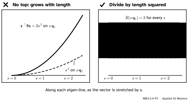
M03.3.4-F5
Wrong beside right. \({\vect{x}\T\mat{S}\vect{x}}\) grows without limit as \(\vect{x}\) gets longer, so it has no largest value. The Rayleigh quotient divides the length out.
“To find the direction of most variance, maximise \({\vect{u}\T\mat{C}\vect{u}}\).”
Not without a rule on the length. Doubling \(\vect{u}\) multiplies \({\vect{u}\T\mat{C}\vect{u}}\) by 4, so the “maximum” runs off to infinity. Either insist that \({\vect{u}\T\vect{u}} = 1\), as PCA does, or divide by \({\vect{u}\T\vect{u}}\) and maximise the Rayleigh quotient. Both give the top eigenvector.
“The largest variance is the largest number on the diagonal of the covariance matrix.”
The diagonal entries are the variances along the coordinate axes: \({\vect{e}_i\T\mat{C}\vect{e}_i} = c_{ii}\). They are values of the Rayleigh quotient, so they lie between \(\lambda_{\min}\) and \(\lambda_{\max}\), and they usually fall short of \(\lambda_{\max}\). For the cloud above, both axes give 2 while the diagonal direction gives 3. An axis wins only when it is an eigenvector, that is, when its variable is uncorrelated with every other variable.
“PCA’s first direction is the eigenvector eigh lists first.”
eigh lists eigenvalues in ascending order, so its first column belongs to the smallest eigenvalue: the direction of least variance. Take the last column, vecs[:, -1], or sort in decreasing order and move the columns with the eigenvalues.
Check yourself
Recall
1. Define the Rayleigh quotient, and say why it depends only on the direction of \(\vect{x}\).
Show answer
\({R(\vect{x})} = {{\vect{x}\T\mat{S}\vect{x}}/{\vect{x}\T\vect{x}}}\). Replacing \(\vect{x}\) by \(s\vect{x}\) multiplies top and bottom by \(s^2\), which cancels.
2. In eigen-coordinates \(\vect{x} = {\sum_i c_i\vect{q}_i}\), what is \({R(\vect{x})}\)?
Show answer
\({\sum_i \lambda_ic_i^2 / \sum_i c_i^2}\), a weighted average of the eigenvalues with weights proportional to \(c_i^2\).
3. Between which two numbers does \(R\) always lie, and where are they reached?
Show answer
Between \(\lambda_{\min}\) and \(\lambda_{\max}\), reached exactly at the eigenvectors for those eigenvalues.
4. What is \({\vect{u}\T\mat{C}\vect{u}}\) for a covariance matrix \(\mat{C}\) and a unit vector \(\vect{u}\)?
Show answer
The variance of the data’s shadows on the line of \(\vect{u}\): the variance of the numbers \({\vect{u} \cdot \vect{x}_k}\).
5. What are \({R(1, 0)}\), \({R(1, 1)}\) and \({R(3, 1)}\) for the running \(\mat{S}\)?
Show answer
2, 3 and 2.6.
Exercises
1.★ Compute \({R(2, -1)}\) for the running \(\mat{S}\) by multiplying out, then check it with the weights \(c_1^2\) and \(c_2^2\).
Show solution
\({\mat{S}\,(2, -1)} = {(4 - 1,\; 2 - 2)} = {(3, 0)}\), so \({\vect{x}\T\mat{S}\vect{x}} = 6\), and \({\vect{x}\T\vect{x}} = 5\). So \(R = {6/5} = 1.2\).
Weights: \(c_1 = {(2 - 1)/\sqrt2}\), so \(c_1^2 = {\tfrac12}\); \(c_2 = {(2 + 1)/\sqrt2}\), so \(c_2^2 = {\tfrac92}\). They add to 5. Then \(R = {(3 \cdot \tfrac12 + 1 \cdot \tfrac92)/5} = {6/5}\). The vector lies mostly along \(\vect{q}_2\), so \(R\) is near the bottom of the band.
2.★★ For the running saddle \(\begin{bmatrix} 1 & 2 \\ 2 & 1 \end{bmatrix}\), with eigenvalues 3 and \({-1}\), find a non-zero vector with \({R(\vect{x})} = 0\).
Show solution
We need \({x^2 + 4xy + y^2} = 0\). Take \(y = 1\): then \({x^2 + 4x + 1} = 0\), so \(x = {-2 \pm \sqrt3}\). For example \(\vect{x} = {(-2 + \sqrt3,\; 1)}\).
The weights explain it: \(R = 0\) needs \({3w_1 - w_2} = 0\) with \({w_1 + w_2} = 1\), so \(w_1 = {\tfrac14}\): one quarter of the weight on the eigenvalue 3 and three quarters on \({-1}\). Because the eigenvalues have opposite signs, the quotient passes through 0. That is the saddle shape of module M03.4.
3.★★★ Let \(\mat{C}\) be a 2 by 2 covariance matrix and \(\vect{u}\), \(\vect{w}\) any two perpendicular unit vectors. Show that the variances along them add up to the trace of \(\mat{C}\), whichever pair is chosen.
Show solution
Write \(\vect{u} = {a\vect{q}_1 + b\vect{q}_2}\) with \({a^2 + b^2} = 1\). The unit vectors perpendicular to \(\vect{u}\) are \({\pm(-b\vect{q}_1 + a\vect{q}_2)}\), since their dot product with \(\vect{u}\) is \({-ab + ba} = 0\); the sign does not change a variance. By Step 2,
The sum of the eigenvalues is the trace (lesson M03.1.3). So the total variance is fixed; turning the axes only moves it from one to the other, and the eigenvectors are the pair that pushes as much as possible onto one axis.
Summary card
The Rayleigh quotient is a weighted average of the eigenvalues, so the eigenvectors are the extreme directions.
M03.3.4-F1
Trapped between the eigenvalues.
Definition.\({R(\vect{x})} = {{\vect{x}\T\mat{S}\vect{x}}/{\vect{x}\T\vect{x}}}\); only the direction counts.
Bounds.\({\lambda_{\min} \le R \le \lambda_{\max}}\), reached at the matching eigenvectors.
Data.\({\vect{u}\T\mat{C}\vect{u}}\) is the variance along \(\vect{u}\); the top eigenvector is the first principal component.
Running example.\(R = {2 + \sin 2\theta}\) for \(\mat{S}\), and \({R(3, 1)} = 2.6\).
Sources and next steps
Sources. Each was opened and checked against this lesson on 15 November 2026.
Marc Peter Deisenroth, A. Aldo Faisal and Cheng Soon Ong, Mathematics for Machine Learning (free PDF), Section 10.2, the maximum variance perspective. Equations (10.9a) and (10.9b) show that the variance of the data projected onto \(\vect{b}_1\) is \({\vect{b}_1\T\mat{S}\vect{b}_1}\); the text notes that a vector twice as long gives up to four times the variance, so it restricts to \({\norm{\vect{b}_1}^2 = 1}\); and (10.13) to (10.15) find that the best \(\vect{b}_1\) is the eigenvector of the largest eigenvalue, which equals the variance. The book divides by \(N\) where this course divides by \({n - 1}\); the direction is the same.
David Austin, Understanding Linear Algebra, Symmetric matrices and variance (open textbook). The variance of the data projected onto a unit vector \(\vect{u}\) is \({\vect{u} \cdot \mat{C}\vect{u}}\), and for a unit eigenvector of \(\mat{C}\) it equals the eigenvalue.
Min-max theorem, Wikipedia, section “Min-max theorem” under “Matrices”. The Courant-Fischer characterisation of each eigenvalue of a Hermitian matrix as a max-min of \({\langle \vect{x}, \mat{A}\vect{x}\rangle}\) over subspaces, and the statement that the largest and smallest values of the Rayleigh quotient are the largest and smallest eigenvalues.
Gilbert Strang, Symmetric matrices and positive definiteness, MIT OpenCourseWare 18.06SC, lecture 25: the lecture that leads from symmetric matrices to the signs of their eigenvalues, the subject of the next module.
NumPy reference, numpy.linalg.eigh (eigenvalues in ascending order) and numpy.cov (with rowvar=False each column is a variable; the default divides by \({n - 1}\)).
Next. Module M03.4 asks when \(R\) is positive in every direction, the positive definite matrices, and draws \({\vect{x}\T\mat{S}\vect{x}}\) as a bowl or a saddle. Module M03.6 turns this lesson’s top direction into principal component analysis.