Every real symmetric matrix factors as S = Q Lambda Q-transpose with Q orthogonal: turn into the eigenbasis, stretch along the axes, turn back. Prove it for 2 by 2 in full, see the induction for any size, handle repeated eigenvalues with Gram-Schmidt, and check it with numpy.linalg.eigh.
M03.3.2L2 Intermediate25 minIn review (what this means)
The maths and code on this page are checked by automated tests on every change, but an independent reader has not signed it off yet. Spot a mistake or a confusing step? Tell us.
State the spectral theorem and explain why Q-transpose can replace Q inverse in the diagonalisation of a symmetric matrix.
Prove the theorem for a symmetric 2 by 2 matrix, and outline the induction that proves it for any size.
Read S = Q Lambda Q-transpose as turn, stretch along the axes, turn back, and predict the ellipse that S makes of the unit circle.
Find an orthonormal basis of eigenvectors when an eigenvalue repeats, using Gram-Schmidt inside the eigenspace.
Use numpy.linalg.eigh correctly: ascending eigenvalues, orthonormal columns, and only one triangle of the matrix read.
The question
Diagonalising a matrix, \(\mat{A} = {\mat{P}\mat{D}\mat{P}^{-1}}\), needs an inverse, and it fails outright for the shear. For a symmetric matrix the last lesson found eigenvectors at right angles. Is that enough to diagonalise every symmetric matrix, with no inverse to compute, and what does the result say a covariance matrix does to space?
From the last lesson
1. Why must eigenvectors for different eigenvalues of a symmetric matrix be perpendicular?
Show answer
By the swap rule, \({\lambda_1 (\vect{v}_1 \cdot \vect{v}_2)} = {\lambda_2 (\vect{v}_1 \cdot \vect{v}_2)}\), and \({\lambda_1 \neq \lambda_2}\) forces the dot product to be zero.
2. What is the discriminant of the characteristic polynomial of \(\begin{bmatrix} a & b \\ b & c \end{bmatrix}\), and why is it never negative?
Show answer
\({(a - c)^2 + 4b^2}\), a sum of two squares.
Intuition
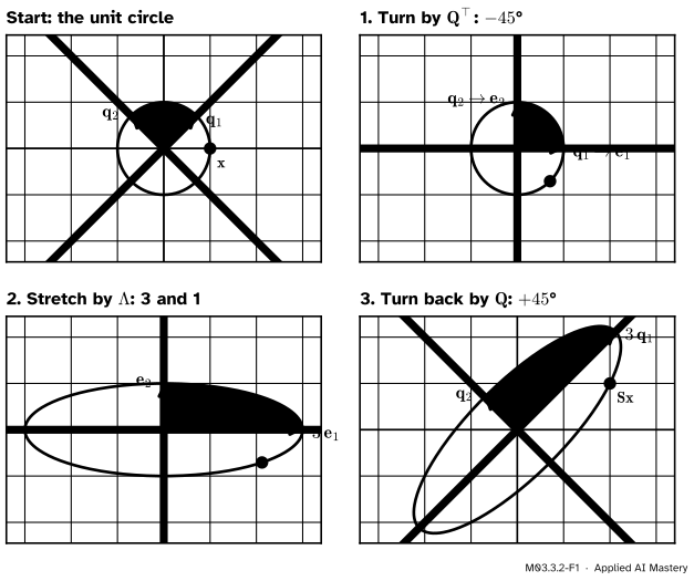
Put unit eigenvectors that are perpendicular to one another into the columns of a matrix \(\mat{Q}\). That matrix is orthogonal (lesson M02.10.2): it turns the plane, or turns it over, without changing any length. The spectral theorem says that every symmetric matrix acts in three plain steps.
M03.3.2-F1
\(\mat{S} = \mat{Q}\mat{\Lambda}\mat{Q}\T\) for the running \(\mat{S}\), read from right to left. Turn the eigenvectors onto the axes, stretch by 3 and 1 along the axes, turn back. The unit circle ends as an ellipse whose axes are the eigenvectors.
The three steps are the whole theorem.
Turn into the eigenbasis, with \(\mat{Q}\T\). The eigenvectors land on the coordinate axes.
Stretch along the axes, with the diagonal matrix \(\mat{\Lambda}\) of eigenvalues. Nothing is mixed, nothing is turned.
Turn back, with \(\mat{Q}\).
A circle survives both turns unchanged, so the only change of shape comes from the stretch. That is why a symmetric matrix makes an ellipse of the unit circle, with its axes along the eigenvectors and its half-widths equal to \(\abs{\lambda_1}\) and \(\abs{\lambda_2}\) (an ellipse squashed flat when an eigenvalue is 0).
Build it up
Step 1. Eigenvectors in the columns. Let \(\vect{q}_1\) and \(\vect{q}_2\) be unit eigenvectors of \(\mat{S}\) with \(\mat{S}\vect{q}_i = \lambda_i\vect{q}_i\), and let \(\mat{Q}\) hold them as columns. Column \(i\) of \(\mat{S}\mat{Q}\) is \(\mat{S}\vect{q}_i = \lambda_i\vect{q}_i\), and column \(i\) of \(\mat{Q}\mat{\Lambda}\) is \(\mat{Q}\) times \(\lambda_i\vect{e}_i\), which is also \(\lambda_i\vect{q}_i\). So
\[
\mat{S}\mat{Q} = \mat{Q}\mat{\Lambda}.
\]
This is the same column-by-column argument as \(\mat{A}\mat{P} = \mat{P}\mat{D}\) in module M03.2.
Step 2. The inverse is free. Entry \(ij\) of \(\mat{Q}\T\mat{Q}\) is \({\vect{q}_i \cdot \vect{q}_j}\): 1 when \(i = j\), because each column has length 1, and 0 otherwise, because the columns are perpendicular. So \(\mat{Q}\T\mat{Q} = \mat{I}\) and \({\mat{Q}^{-1}} = \mat{Q}\T\). Multiply \(\mat{S}\mat{Q} = \mat{Q}\mat{\Lambda}\) on the right by \(\mat{Q}\T\):
(The first equality uses \(\mat{Q}\mat{Q}\T = \mat{I}\), which holds because a square matrix’s left inverse is also its right inverse.)
Step 3. Read it as three moves. Applied to a vector, \({\mat{Q}\T\vect{x}}\) has entries \({\vect{q}_1 \cdot \vect{x}}\) and \({\vect{q}_2 \cdot \vect{x}}\): the coordinates of \(\vect{x}\) in the eigenbasis (lesson M02.10.1). \(\mat{\Lambda}\) multiplies each coordinate by its eigenvalue. \(\mat{Q}\) rebuilds a vector from the new coordinates. In one line,
Step 4. Why the image is an ellipse. Take \(\vect{x}\) on the unit circle. Then \(\vect{y} = \mat{Q}\T\vect{x}\) is on the unit circle too, since \(\mat{Q}\T\) keeps lengths: \({y_1^2 + y_2^2} = 1\). After the stretch, \(z_1 = {\lambda_1 y_1}\) and \(z_2 = {\lambda_2 y_2}\), so
an ellipse with half-widths \(\abs{\lambda_1}\) and \(\abs{\lambda_2}\) along the axes (both eigenvalues non-zero). The last turn by \(\mat{Q}\) carries those axes onto \(\vect{q}_1\) and \(\vect{q}_2\). A negative eigenvalue flips its axis, so with one negative eigenvalue the ellipse is traced the other way round (two flips make a half-turn, which keeps the direction); an eigenvalue 0 squashes the ellipse flat onto a segment.
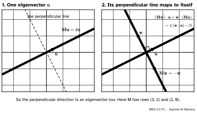
Step 5. Why the second eigenvector always exists. The last lesson’s exercise 3 is the heart of the proof. Once one unit eigenvector \(\vect{u}\) is known, every \(\vect{w}\) perpendicular to it is sent to a vector that is still perpendicular to it.
M03.3.2-F2
The 2 by 2 proof in two frames, on the matrix \(\mat{M}\) of the last lesson. The line perpendicular to one eigenvector is carried into itself, so a vector on it can only be stretched or flipped: it is a second eigenvector.
The formal statement
NoteThe spectral theorem
Let \(\mat{S}\) be a real symmetric \({n \times n}\) matrix. Then there is an orthogonal matrix \(\mat{Q}\) and a real diagonal matrix \(\mat{\Lambda}\) with
\[
\mat{S} = \mat{Q}\mat{\Lambda}\mat{Q}\T .
\]
The columns \({\vect{q}_1, \dots, \vect{q}_n}\) of \(\mat{Q}\) are orthonormal eigenvectors of \(\mat{S}\), and the diagonal entries \({\lambda_1, \dots, \lambda_n}\) of \(\mat{\Lambda}\) are the matching eigenvalues. Conversely, every matrix of the form \(\mat{Q}\mat{\Lambda}\mat{Q}\T\) is symmetric.
The converse takes one line, because transposing reverses the order of a product and a diagonal matrix is its own transpose:
So the symmetric matrices are exactly the matrices that have an orthonormal basis of eigenvectors.
Proof for 2 by 2. Let \(\mat{S}\) be real, symmetric and 2 by 2.
By the last lesson its eigenvalues are real. Take one, \(\lambda_1\).
\({\mat{S} - \lambda_1\mat{I}}\) is a real matrix with determinant 0, so its null space contains a real non-zero vector (lesson M02.7). Divide it by its length to get a unit eigenvector \(\vect{q}_1 = {(p, r)}\).
Let \(\vect{q}_2 = {(-r, p)}\). It has length 1 and \({\vect{q}_1 \cdot \vect{q}_2} = {-pr + rp} = 0\).
By the swap rule, \({(\mat{S}\vect{q}_2) \cdot \vect{q}_1} = {\vect{q}_2 \cdot (\lambda_1\vect{q}_1)} = 0\). So \(\mat{S}\vect{q}_2\) is perpendicular to \(\vect{q}_1\). In the plane, the vectors perpendicular to \(\vect{q}_1\) form the single line through \(\vect{q}_2\), so \(\mat{S}\vect{q}_2 = \lambda_2\vect{q}_2\) for some number \(\lambda_2\).
Now Steps 1 and 2 of the build give \(\mat{S} = \mat{Q}\mat{\Lambda}\mat{Q}\T\) with \(\mat{Q} = {[\,\vect{q}_1\ \vect{q}_2\,]}\) and \(\mat{\Lambda} = {\operatorname{diag}(\lambda_1, \lambda_2)}\). \(\blacksquare\)
Nothing in the proof asked the eigenvalues to differ. If \(\lambda_2 = \lambda_1\), the matrix is \(\lambda_1\mat{I}\) and every orthonormal pair works.
A repeated eigenvalue in 3 by 3. Take \(\mat{S}_3 = \begin{bmatrix} 2 & 1 & 1 \\ 1 & 2 & 1 \\ 1 & 1 & 2 \end{bmatrix}\). Then \({\mat{S}_3(1, 1, 1)} = {(4, 4, 4)}\), so 4 is an eigenvalue with \(\vect{q}_1 = {(1, 1, 1)/\sqrt{3}}\). And \({\mat{S}_3 - \mat{I}}\) is the matrix of all ones, which sends \(\vect{x}\) to zero exactly when \({x_1 + x_2 + x_3} = 0\). So the eigenvalue 1 has a whole plane of eigenvectors, the eigenspace. Two natural choices in it, \({(1, -1, 0)}\) and \({(1, 0, -1)}\), lean at 60 degrees, since their dot product is 1 and each has length \({\sqrt{2}}\). Every combination of eigenvectors for 1 is again an eigenvector for 1, so Gram-Schmidt (lesson M02.10.3) can straighten them without leaving the plane:
Here \({\tfrac{1}{\sqrt{2}}}\) is \({\vect{q}_2 \cdot (1, 0, -1)}\), and \(\norm{\vect{e}} = {\sqrt{\tfrac14 + \tfrac14 + 1}} = {\sqrt{3/2}}\).
M03.3.2-F3
With the eigenvalue 1 repeated, any two vectors of the plane \({x + y + z} = 0\) are eigenvectors. Gram-Schmidt picks a perpendicular pair inside the plane, and \(\vect{q}_1\) is perpendicular to the whole plane by the last lesson.
Mathematics for Machine Learning works the same example scaled: its matrix \(\begin{bmatrix} 3 & 2 & 2 \\ 2 & 3 & 2 \\ 2 & 2 & 3 \end{bmatrix}\) is \({2\mat{S}_3 - \mat{I}}\), with eigenvalues \({2 \cdot 4 - 1} = 7\) and \({2 \cdot 1 - 1} = 1\) and the same eigenvectors.
Go deeper: the proof for n by n, by induction on the size
Suppose the theorem holds for all symmetric matrices of size \({n - 1}\), and let \(\mat{S}\) be symmetric of size \(n\).
One eigenvector. The characteristic polynomial has a root \(\lambda_1\), possibly complex, by the fundamental theorem of algebra. By the last lesson it is real. Then \({\mat{S} - \lambda_1\mat{I}}\) is real and singular, so it has a real unit null vector \(\vect{q}_1\).
The rest of space is carried into itself. Let \(W\) be the set of vectors perpendicular to \(\vect{q}_1\), a subspace of dimension \({n - 1}\). For \(\vect{w}\) in \(W\), the swap rule gives \({(\mat{S}\vect{w}) \cdot \vect{q}_1} = {\lambda_1 (\vect{w} \cdot \vect{q}_1)} = 0\), so \(\mat{S}\vect{w}\) is in \(W\) too.
A smaller symmetric matrix. Pick an orthonormal basis of \(W\) (Gram-Schmidt) and put it in the columns of an \({n \times (n - 1)}\) matrix \(\mat{U}\). Then \(\mat{U}\T\mat{U} = \mat{I}\), and \(\mat{U}\mat{U}\T\vect{w} = \vect{w}\) for every \(\vect{w}\) in \(W\), because \(\mat{U}\T\vect{w}\) lists the coordinates of \(\vect{w}\) in that basis and \(\mat{U}\) rebuilds it. Let \(\mat{B} = \mat{U}\T\mat{S}\mat{U}\). It is symmetric, since \({\mat{B}\T} = {\mat{U}\T\mat{S}\T\mat{U}} = \mat{B}\), and of size \({n - 1}\), so by the induction hypothesis \(\mat{B} = \mat{V}\mat{\Lambda}'\mat{V}\T\) with \(\mat{V}\) orthogonal.
Back in the big space. Each column of \(\mat{S}\mat{U}\) lies in \(W\), so \(\mat{S}\mat{U} = \mat{U}\mat{U}\T\mat{S}\mat{U} = \mat{U}\mat{B}\). Then
So the \({n - 1}\) columns of \(\mat{U}\mat{V}\) are eigenvectors of \(\mat{S}\). They are orthonormal, because \({(\mat{U}\mat{V})\T(\mat{U}\mat{V})} = {\mat{V}\T\mat{U}\T\mat{U}\mat{V}} = \mat{I}\), and they lie in \(W\), so they are perpendicular to \(\vect{q}_1\). With \(\vect{q}_1\) in front they fill an orthogonal \(\mat{Q}\) with \(\mat{S}\mat{Q} = \mat{Q}\mat{\Lambda}\), and \(\mat{\Lambda}\) has \(\lambda_1\) followed by the diagonal of \(\mat{\Lambda}'\). The case \(n = 1\) is trivial, so the theorem holds for every size. \(\blacksquare\)
Axler (result 7.29) reaches the same theorem by a different road: his results 6.37 and 7.27 give an upper triangular matrix in some orthonormal basis (the idea behind Schur’s theorem, his 6.38), and a triangular matrix that is also symmetric must be diagonal.
Worked example
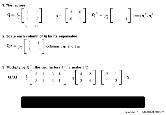
Write \(\mat{S} = \begin{bmatrix} 2 & 1 \\ 1 & 2 \end{bmatrix}\) as \(\mat{Q}\mat{\Lambda}\mat{Q}\T\) and check every factor.
The last lesson found \(\lambda_1 = 3\), \(\lambda_2 = 1\) and the orthonormal eigenvectors \(\vect{q}_1 = {(1, 1)/\sqrt{2}}\), \(\vect{q}_2 = {(1, -1)/\sqrt{2}}\).
M03.3.2-F4
The spectral factorisation of \(\mat{S}\) multiplied out by hand.
The factors.\(\mat{Q} = \tfrac{1}{\sqrt{2}}\begin{bmatrix} 1 & 1 \\ 1 & -1 \end{bmatrix}\) and \(\mat{\Lambda} = \begin{bmatrix} 3 & 0 \\ 0 & 1 \end{bmatrix}\). This \(\mat{Q}\) happens to equal its own transpose.
The product. Scaling the columns of \(\mat{Q}\) by 3 and 1 gives \(\mat{Q}\mat{\Lambda} = \tfrac{1}{\sqrt{2}}\begin{bmatrix} 3 & 1 \\ 3 & -1 \end{bmatrix}\). Then
Turn or turn-over?\(\det\mat{Q} = {\tfrac12\,(-1 - 1)} = {-1}\), so this \(\mat{Q}\) is a reflection (lesson M02.10.2). Replace \(\vect{q}_2\) by \({-\vect{q}_2} = {(-1, 1)/\sqrt{2}}\), still a unit eigenvector, and \(\det\mat{Q} = {+1}\): a turn by 45 degrees. The factorisation still holds, since \({\lambda_2(-\vect{q}_2)(-\vect{q}_2)\T} = {\lambda_2\vect{q}_2\vect{q}_2\T}\). The anchor figure uses this turn; either choice is correct.
One vector, three moves. For \(\vect{x} = {(1, 0)}\): \(\mat{Q}\T\vect{x} = {(\vect{q}_1 \cdot \vect{x},\; \vect{q}_2 \cdot \vect{x})} = {(1/\sqrt{2},\; 1/\sqrt{2})}\); the stretch gives \({(3/\sqrt{2},\; 1/\sqrt{2})}\); and
which is \({\mat{S}\,(1, 0)}\), the first column of \(\mat{S}\).
Code
From scratch: build \(\mat{Q}\) and \(\mat{\Lambda}\) for a symmetric 2 by 2 matrix from the formulas of the last lesson, then run Gram-Schmidt inside the repeated eigenspace of \(\mat{S}_3\).
import mathimport numpy as npdef spectral_2x2(a, b, c):"""Q (orthonormal eigenvector columns) and the eigenvalues of [[a, b], [b, c]], larger first.""" centre, half = (a + c) /2, math.sqrt((a - c) **2+4* b **2) /2 lam1, lam2 = centre + half, centre - half v = np.array([b, lam1 - a]) if b !=0else (np.array([1.0, 0.0]) if a >= c else np.array([0.0, 1.0])) q1 = v / np.linalg.norm(v) q2 = np.array([-q1[1], q1[0]]) # q1 turned by 90 degrees: the proof's step 3return np.column_stack([q1, q2]), np.array([lam1, lam2])for a, b, c in [(2, 1, 2), (3, 2, 0), (1, 2, 1), (5, 0, 5)]: Q, lam = spectral_2x2(a, b, c) S = np.array([[a, b], [b, c]], dtype=float)print((a, b, c), "eigenvalues", lam, " Q^T Q = I:", np.allclose(Q.T @ Q, np.eye(2))," Q diag Q^T = S:", np.allclose(Q @ np.diag(lam) @ Q.T, S))
The library routine for this job is np.linalg.eigh. It returns the eigenvalues in ascending order and the orthonormal eigenvectors as columns, so its \(\mat{Q}\) may list \(\vect{q}_2\) before \(\vect{q}_1\) and may flip any column’s sign. Those are free choices, and the checks below do not depend on them.
for name, M in [("S", np.array([[2.0, 1.0], [1.0, 2.0]])), ("S3", S3)]: lam, Q = np.linalg.eigh(M)print(name, "eigh eigenvalues:", lam.round(10)," orthonormal:", np.allclose(Q.T @ Q, np.eye(len(M)))," rebuilds M:", np.allclose(Q @ np.diag(lam) @ Q.T, M))lam_eig, P = np.linalg.eig(S3) # the general routine: no promise of order or orthogonalityprint("eig eigenvalues of S3:", lam_eig.round(10))
eig finds the same eigenvalues, in an order it does not promise. For a repeated eigenvalue it may return two eigenvectors that lean, because it does not know the matrix is symmetric. Use eigh for symmetric matrices: it is faster and its columns are always orthonormal.
Explore
M03.3-X1
Spectral ellipse
Move the three sliders to set the entries \(a\), \(b\) and \(c\) of a symmetric matrix. The unit circle, its image and the two eigenvectors are drawn, with each eigenvalue printed on its axis. Switch on Pieces to split the matrix into its two rank-one parts and see what each does to the vector you choose with the angle slider.
Things to try:
Start from \(a = c = 2\), \(b = 1\), the running \(\mat{S}\). Read the half-widths 3 and 1 off the axes.
Move \(b\) from 1 to \({-1}\). The ellipse swings to the other diagonal; the eigenvectors stay square.
Set \(a = c\) and \(b = 0\). The ellipse becomes a circle: a repeated eigenvalue, and every direction is an eigenvector.
Make \({ac < b^2}\), for example \(a = c = 1\), \(b = 2\) (the running saddle). One eigenvalue turns negative and that axis flips, so the image is traced the other way round.
Pitfalls
M03.3.2-F5
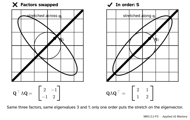
Wrong beside right, with the turn \(\mat{Q}\) whose columns are \(\vect{q}_1\) and \({(-1, 1)/\sqrt{2}}\). Swapping the outer factors stretches the circle across the eigenvector instead of along it.
“\(\mat{Q}\T\mat{\Lambda}\mat{Q}\) and \(\mat{Q}\mat{\Lambda}\mat{Q}\T\) are the same thing.”
Not in general. They agree when \(\mat{Q}\) happens to be symmetric, as the course’s \(\tfrac{1}{\sqrt{2}}\begin{bmatrix} 1 & 1 \\ 1 & -1 \end{bmatrix}\) is, but the eigenvectors are the columns of \(\mat{Q}\), so \(\mat{Q}\) goes on the left. With the turn by 45 degrees, \(\mat{Q}\T\mat{\Lambda}\mat{Q} = \begin{bmatrix} 2 & -1 \\ -1 & 2 \end{bmatrix}\), a different matrix. Check by multiplying \(\mat{Q}\mat{\Lambda}\mat{Q}\T\vect{q}_1\): it gives \(\lambda_1\vect{q}_1\).
“I can sort the eigenvalues and keep the eigenvectors where they were.”
Each eigenvalue belongs to its own column. eigh returns 1 before 3; if you reverse the eigenvalues to put the largest first, reverse the columns of \(\mat{Q}\) too (lam[::-1], Q[:, ::-1]). Otherwise \(\mat{Q}\mat{\Lambda}\mat{Q}\T\) is the wrong matrix, here the factors-swapped one of the figure.
“eigh will complain if my matrix is not symmetric.”
It does not check. By default it reads only the lower triangle and assumes the upper one mirrors it. Handed the running \(\mat{A} = \begin{bmatrix} 4 & 1 \\ 2 & 3 \end{bmatrix}\), it silently answers for \(\begin{bmatrix} 4 & 2 \\ 2 & 3 \end{bmatrix}\), with eigenvalues \({(7 \pm \sqrt{17})/2}\), about 5.56 and 1.44, instead of 5 and 2. A covariance matrix built in floating point can also be off by a last digit; symmetrise it with \({(\mat{C} + \mat{C}\T)/2}\) if in doubt.
Check yourself
Recall
1. State the spectral theorem.
Show answer
Every real symmetric matrix can be written \(\mat{S} = \mat{Q}\mat{\Lambda}\mat{Q}\T\), with \(\mat{Q}\) orthogonal (its columns orthonormal eigenvectors) and \(\mat{\Lambda}\) real and diagonal (the eigenvalues).
2. Why does \(\mat{Q}\T\) appear where \({\mat{P}^{-1}}\) appears in \(\mat{A} = {\mat{P}\mat{D}\mat{P}^{-1}}\)?
Show answer
Because the columns of \(\mat{Q}\) are orthonormal, so \(\mat{Q}\T\mat{Q} = \mat{I}\) and \({\mat{Q}^{-1}} = \mat{Q}\T\).
3. Read \(\mat{S}\vect{x} = \mat{Q}\mat{\Lambda}\mat{Q}\T\vect{x}\) as three moves.
Show answer
Turn into the eigenbasis (coordinates \({\vect{q}_i \cdot \vect{x}}\)), stretch each coordinate by its eigenvalue, turn back.
4. What does a symmetric 2 by 2 matrix with eigenvalues 3 and 1 do to the unit circle?
Show answer
It makes an ellipse with half-widths 3 and 1, whose axes lie along the two eigenvectors.
5. An eigenvalue repeats and its eigenvectors fill a plane. How do you get perpendicular unit eigenvectors in it?
Show answer
Take any two independent eigenvectors in the plane and run Gram-Schmidt on them. Combinations of eigenvectors for one eigenvalue are still eigenvectors, so the results stay in the plane.
Exercises
1.★ Write the running saddle \(\begin{bmatrix} 1 & 2 \\ 2 & 1 \end{bmatrix}\) as \(\mat{Q}\mat{\Lambda}\mat{Q}\T\) and multiply it out to check.
Show solution
Its eigenvalues are 3 and \({-1}\) with unit eigenvectors \({(1, 1)/\sqrt{2}}\) and \({(1, -1)/\sqrt{2}}\) (last lesson, exercise 2). So \(\mat{Q} = \tfrac{1}{\sqrt{2}}\begin{bmatrix} 1 & 1 \\ 1 & -1 \end{bmatrix}\) and \(\mat{\Lambda} = {\operatorname{diag}(3, -1)}\). Then \(\mat{Q}\mat{\Lambda} = \tfrac{1}{\sqrt{2}}\begin{bmatrix} 3 & -1 \\ 3 & 1 \end{bmatrix}\) and
Check: the trace is \({25/25} = 1 = {2 + (-1)}\), and \({\mat{S}\,(3, 4)} = {\tfrac{1}{25}(6 + 144,\; 108 + 92)} = {(6, 8)}\), which is \({2\,(3, 4)}\).
3.★★★ Show that a symmetric matrix whose only eigenvalue is \(\lambda\) must be \(\lambda\mat{I}\). Then explain why the shear \(\begin{bmatrix} 1 & 1 \\ 0 & 1 \end{bmatrix}\), whose only eigenvalue is 1, cannot be symmetric, and why this does not contradict anything.
Show solution
By the spectral theorem \(\mat{S} = \mat{Q}\mat{\Lambda}\mat{Q}\T\), and here every diagonal entry of \(\mat{\Lambda}\) is \(\lambda\), so \(\mat{\Lambda} = \lambda\mat{I}\). Then \({\mat{S}} = {\lambda\mat{Q}\mat{Q}\T} = {\lambda\mat{I}}\).
The shear has 1 as its only eigenvalue but is not the identity, so by the first part it cannot be symmetric, and indeed its off-diagonal entries are 1 and 0. There is no contradiction: the shear has only one line of eigenvectors, so it cannot be diagonalised at all (module M03.2), and the spectral theorem says nothing about matrices that are not symmetric.
Summary card
Every symmetric matrix is a turn, a stretch along the axes and a turn back.
M03.3.2-F1
Turn, stretch, turn back.
Spectral theorem.\(\mat{S} = \mat{Q}\mat{\Lambda}\mat{Q}\T\), with \(\mat{Q}\T\mat{Q} = \mat{I}\).
Columns.\(\mat{S}\vect{q}_i = \lambda_i\vect{q}_i\), so \(\mat{S}\mat{Q} = \mat{Q}\mat{\Lambda}\).
Ellipse. The unit circle goes to an ellipse with half-widths \(\abs{\lambda_i}\) along \(\vect{q}_i\).
Repeated eigenvalue. Gram-Schmidt inside the eigenspace.
Sources. Each was opened and checked against this lesson on 15 November 2026.
Sheldon Axler, Linear Algebra Done Right, 4th edition (open access). Result 7.29, the real spectral theorem: an operator on a real inner product space is self-adjoint exactly when it has a diagonal matrix in some orthonormal basis, exactly when the space has an orthonormal basis of its eigenvectors. Its proof goes through an upper-triangular matrix in an orthonormal basis (6.37, the result behind Schur’s theorem 6.38) and the minimal polynomial of a self-adjoint operator (7.27). Example 7.30 is a 3 by 3 symmetric matrix with eigenvectors \({(1, -1, 0)/\sqrt{2}}\), \({(1, 1, 1)/\sqrt{3}}\) and \({(1, 1, -2)/\sqrt{6}}\), the same three directions as here.
Marc Peter Deisenroth, A. Aldo Faisal and Cheng Soon Ong, Mathematics for Machine Learning (free PDF), Section 4.2. Theorem 4.15, the spectral theorem, and Example 4.8: the matrix with 3 on the diagonal and 2 elsewhere, eigenvalues 1 (repeated) and 7, whose eigenspace for 1 is made orthogonal with Gram-Schmidt.
Gilbert Strang, Symmetric matrices and positive definiteness, MIT OpenCourseWare 18.06SC, lecture 25 and its lecture summary: a symmetric matrix can be written \({\mat{Q}\mat{\Lambda}\mat{Q}^{-1}} = {\mat{Q}\mat{\Lambda}\mat{Q}\T}\) with \(\mat{Q}\) orthogonal, which mathematicians call the spectral theorem and mechanics the principal axis theorem; and any matrix of that form is symmetric.
NumPy reference, numpy.linalg.eigh. Eigenvalues in ascending order, normalised eigenvectors in columns, and the UPLO argument: the lower triangle is used by default.
Next.M03.3.3 A sum of rank-one pieces multiplies \(\mat{Q}\mat{\Lambda}\mat{Q}\T\) out column by row, and finds that a symmetric matrix is a weighted sum of projections onto perpendicular lines.