A map that turns every vector has no real eigenvector, but its characteristic equation still has roots: a complex conjugate pair. Read their modulus as a stretch and their argument as a turn, find the basis in which the running map T is a plain turn and stretch, and see why repeated application spirals.
M03.1.4L2 Intermediate25 minIn review (what this means)
The maths and code on this page are checked by automated tests on every change, but an independent reader has not signed it off yet. Spot a mistake or a confusing step? Tell us.
Show that a rotation by an angle theta has the eigenvalues e to the i theta and e to the minus i theta, and no real eigenvector unless theta is a multiple of 180 degrees.
Find the complex eigenvalues of a 2 by 2 matrix and read their modulus as a stretch and their argument as a turn.
Derive the basis, made of the real and imaginary parts of an eigenvector, in which the running map T is the square root of 3 times a 30-degree turn, and check it by multiplication.
Use the spectral radius to predict whether repeated application of a matrix shrinks, keeps or grows vectors, as in a recurrent network.
The question
Ask NumPy for the eigenvalues of the running map \({T(x, y)} = {(x + y,\; -x + 2y)}\) and it answers about 1.5+0.866j and 1.5-0.866j. A real matrix that moves real vectors has complex eigenvalues. What do they mean, and why does the same kind of number decide whether a recurrent neural network’s signal explodes or fades away?
From the last lesson
1. What do the eigenvalues of a square matrix add up to, and what do they multiply to?
Show answer
The trace and the determinant, counted with repeats.
2. If \({\mat{A}\vect{v}} = {\lambda\vect{v}}\), what is the eigenvalue of \(\mat{A}^k\) for \(\vect{v}\)?
Show answer
\(\lambda^k\): each application multiplies by \(\lambda\) once more.
Intuition
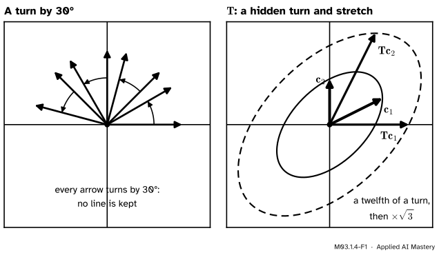
A rotation of the plane turns every non-zero vector, so no vector stays on its line and there is no real eigenvector. The running map \(\mat{T}\), with rows \((1, 1)\) and \((-1, 2)\), also turns every vector (M02.9.4 showed this). Yet the eigenvalue equation still has solutions: complex ones.
M03.1.4-F1
A turn keeps no line (left). The map \(\mat{T}\) keeps no line either, but it hides a turn: it moves each point of the orange ellipse a twelfth of the way round and then stretches the whole ellipse \(\sqrt3\) times (right).
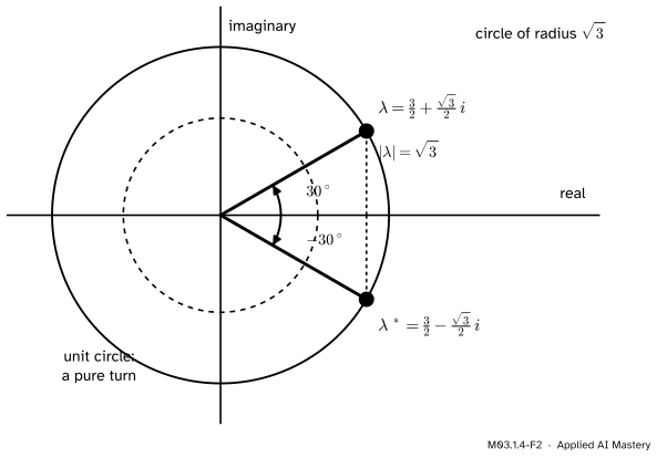
The complex eigenvalue \(\lambda = \frac32 + \frac{\sqrt3}{2}i\) carries both facts. Its modulus, \(\abs{\lambda} = \sqrt3\), is the stretch. Its argument, \(30^\circ\), is the turn, measured not in the standard picture but in a skewed basis built from a complex eigenvector.
Build it up
Step 1. The rotation. The rotation by \(\theta\) is \(\mat{R}(\theta) = \begin{bmatrix} \cos\theta & -\sin\theta \\ \sin\theta & \cos\theta \end{bmatrix}\) (M02.4.3). Its trace is \(2\cos\theta\) and its determinant is \({\cos^2\theta + \sin^2\theta} = 1\), so
which is negative unless \(\sin\theta = 0\), that is unless \(\theta\) is a multiple of \(180^\circ\). The quadratic formula with \({\sqrt{-4\sin^2\theta}} = {2i\sin\theta}\) (taking \(\sin\theta > 0\); the other sign just swaps the two roots) gives
so \(\arg\lambda = 30^\circ\), since \(\lambda\) lies in the first quarter of the plane.
M03.1.4-F2
The eigenvalues of \(\mat{T}\): a conjugate pair, mirror images in the real axis, at distance \(\sqrt3\) from the origin and at angles \(\pm 30^\circ\). A pure rotation would put them on the unit circle.
Step 4. Always a conjugate pair. For a real matrix, take complex conjugates of both sides of \({\mat{A}\vect{v}} = {\lambda\vect{v}}\). The entries of \(\mat{A}\) are real, so they are unchanged, and \({\mat{A}\vect{v}^*} = {\lambda^*\vect{v}^*}\): the conjugate \(\lambda^*\) is an eigenvalue too, with the conjugate eigenvector. A 2 by 2 real matrix therefore has either two real eigenvalues or one conjugate pair (M01.9.4).
The formal statement
NoteTheorem: the rotation-scaling form
Let \(\mat{A}\) be a real 2 by 2 matrix with a non-real eigenvalue \({\lambda = a + bi}\), and let \(\vect{v}\) be an eigenvector. Write \({\vect{v} = \vect{c}_1 + i\,\vect{c}_2}\) with \(\vect{c}_1\), \(\vect{c}_2\) real, and put them in the columns of \(\mat{C}\). Then \(\mat{C}\) is invertible and
\[
\begin{aligned}
\mat{C}^{-1}\mat{A}\mat{C}
&= \begin{bmatrix} a & b \\ -b & a \end{bmatrix} \\
&= r\begin{bmatrix} \cos\theta & \sin\theta \\ -\sin\theta & \cos\theta \end{bmatrix},
\end{aligned}
\]
where \({r = \abs{\lambda}}\) and \({\theta = \arg\lambda}\). The second matrix is \(r\) times a turn by \(\theta\) clockwise, \(r\,\mat{R}(-\theta)\).
Derivation. Multiply out \({\mat{A}\vect{v}} = {\lambda\vect{v}}\) with both sides split into real and imaginary parts:
The coordinates of \(\mat{A}\vect{c}_1\) in the basis \(\vect{c}_1, \vect{c}_2\) are \((a, -b)\) and those of \(\mat{A}\vect{c}_2\) are \((b, a)\). These are the columns of the matrix of the map in that basis, which is \(\mat{C}^{-1}\mat{A}\mat{C}\) (M02.9.3). Finally \(a = r\cos\theta\) and \(b = r\sin\theta\) by the polar form. \(\blacksquare\)
Go deeper: why the real and imaginary parts are independent
Suppose \(\vect{c}_1\) and \(\vect{c}_2\) were dependent. If \(\vect{c}_1 = \vect{0}\), then \({\vect{v} = i\,\vect{c}_2}\), and dividing \({\mat{A}\vect{v}} = {\lambda\vect{v}}\) by \(i\) gives \({\mat{A}\vect{c}_2} = {\lambda\vect{c}_2}\). Otherwise \({\vect{c}_2 = k\,\vect{c}_1}\) for a real \(k\), so \({\vect{v} = (1 + ik)\,\vect{c}_1}\), and dividing by \({1 + ik}\) gives \({\mat{A}\vect{c}_1} = {\lambda\vect{c}_1}\). Either way a non-zero real vector would satisfy \({\mat{A}\vect{w}} = {\lambda\vect{w}}\). The left side is real; the right side has imaginary part \({b\,\vect{w}} \neq \vect{0}\) because \(b \neq 0\). That is impossible, so \(\mat{C}\) is invertible.
Powers spiral. From \({\mat{C}^{-1}\mat{A}\mat{C}} = {r\,\mat{R}(-\theta)}\) we get \({\mat{A}} = {\mat{C}\,r\mat{R}(-\theta)\,\mat{C}^{-1}}\), and in a product of \(k\) copies every inner \({\mat{C}^{-1}\mat{C}}\) cancels:
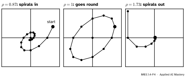
Each application turns by \(\theta\) in the skewed coordinates and stretches by \(r\). In the standard picture the path is a spiral round an ellipse: inwards if \({r < 1}\), closed if \({r = 1}\), outwards if \({r > 1}\).
NoteDefinition: spectral radius
The spectral radius\(\rho(\mat{A})\) is the largest modulus among the eigenvalues of \(\mat{A}\).
For the running matrices, \(\rho(\mat{A}) = 5\), \(\rho(\mat{R}(\theta)) = 1\) and \(\rho(\mat{T}) = \sqrt3 \approx 1.73\). In the long run, repeated application shrinks every vector to zero when \(\rho < 1\) and blows some up when \(\rho > 1\).
M03.1.4-F4
The same turn with three stretches. Scaling \(\mat{T}\) by \(\frac12\) gives \(\rho \approx 0.87\), and the iterates spiral in; by \(\frac{1}{\sqrt3}\) gives \(\rho = 1\), and they go round one ellipse for ever; \(\mat{T}\) itself has \(\rho = \sqrt3\), and they spiral out.
Worked example
Find a complex eigenvector of \(\mat{T}\), build \(\mat{C}\), and check that \(\mat{C}^{-1}\mat{T}\mat{C}\) is \(\sqrt3\) times a \(30^\circ\) turn.
An eigenvector. For \(\lambda = \frac32 + \frac{\sqrt3}{2}i\), the first row of \({\mat{T} - \lambda\mat{I}}\) says \({(1 - \lambda)x + y} = 0\). Choose \(x = 2\); then \({y = 2(\lambda - 1)} = {1 + \sqrt3\,i}\), so \(\vect{v} = (2,\; 1 + \sqrt3\,i)\). Check the second entry of \(\mat{T}\vect{v}\) against \(\lambda\) times the second entry of \(\vect{v}\):
The first entries agree too: \({2 + 1 + \sqrt3\,i} = {3 + \sqrt3\,i} = {2\lambda}\).
The basis. The real and imaginary parts are \({\vect{c}_1 = (2, 1)}\) and \({\vect{c}_2 = (0, \sqrt3)}\), so \({\mat{C}} = \begin{bmatrix} 2 & 0 \\ 1 & \sqrt3 \end{bmatrix}\) and the theorem predicts
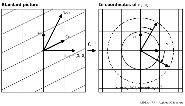
They match. Read column by column: \({\mat{T}\vect{c}_1} = (3, 0)\) and \({\mat{T}\vect{c}_2} = {(\sqrt3,\; 2\sqrt3)}\).
M03.1.4-F3
The same map in two coordinate systems. In standard coordinates \(\mat{T}\) looks lopsided. Measured in the coordinates of \(\vect{c}_1, \vect{c}_2\) it is a plain turn by \(30^\circ\) and a stretch by \(\sqrt3\).
A consequence. Twelve turns of \(30^\circ\) make a full turn, so \({\mat{T}^{12}} = {\mat{C}\,(\sqrt3)^{12}\mat{R}(-360^\circ)\,\mat{C}^{-1}} = {729\,\mat{I}}\): twelve applications of \(\mat{T}\) multiply every vector by exactly \({3^6} = 729\).
Code
NumPy returns the conjugate pair, with the moduli and arguments one call away.
import numpy as npT = np.array([[1.0, 1.0], [-1.0, 2.0]])values, vectors = np.linalg.eig(T)print("eigenvalues:", values)print("modulus:", np.abs(values))print("argument in degrees:", np.degrees(np.angle(values)))print("spectral radius:", np.abs(values).max())
From scratch: build \(\mat{C}\) from the eigenvector of the eigenvalue with positive imaginary part. NumPy scales the eigenvector by some complex number of its choosing, which changes \(\mat{C}\), but the derivation above works for every eigenvector, so the result does not change.
k =int(np.argmax(values.imag)) # the eigenvalue a + bi with b > 0lam, v = values[k], vectors[:, k]C = np.column_stack([v.real, v.imag])B = np.linalg.solve(C, T @ C) # C^-1 T C, without forming the inverseprint("C^-1 T C =\n", B.round(6))r, theta =abs(lam), np.angle(lam)turn = np.array([[np.cos(theta), np.sin(theta)], [-np.sin(theta), np.cos(theta)]])print("sqrt(3) times a clockwise 30-degree turn:\n", (r * turn).round(6))hand = np.array([[2.0, 0.0], [1.0, np.sqrt(3)]])print("hand basis:\n", np.linalg.solve(hand, T @ hand).round(6))print("T^6 =\n", np.linalg.matrix_power(T, 6), "\nT^12 =\n", np.linalg.matrix_power(T, 12))
C^-1 T C =
 [[ 1.5       0.866025]
 [-0.866025  1.5     ]]
sqrt(3) times a clockwise 30-degree turn:
 [[ 1.5       0.866025]
 [-0.866025  1.5     ]]
hand basis:
 [[ 1.5       0.866025]
 [-0.866025  1.5     ]]
T^6 =
 [[-27.   0.]
 [  0. -27.]]
T^12 =
 [[729.   0.]
 [  0. 729.]]
Last, the recurrent-network picture: a hidden state updated by \({\vect{h}_{t+1}} = {\mat{W}\vect{h}_t}\), with no input and no non-linearity, for three scalings of \(\mat{T}\).
h0 = np.array([1.0, 0.0])for name, W in [("T/2", T /2), ("T/sqrt3", T / np.sqrt(3)), ("T", T)]: h, norms = h0, []for t inrange(36): h = W @ h norms.append(np.linalg.norm(h)) rho = np.abs(np.linalg.eig(W).eigenvalues).max()print(f"{name:8s} rho = {rho:.3f} |h_36| = {norms[-1]:.3g} largest |h_t| = {max(norms):.3g}")
T/2      rho = 0.866   |h_36| = 0.00564   largest |h_t| = 0.839
T/sqrt3  rho = 1.000   |h_36| = 1   largest |h_t| = 1.41
T        rho = 1.732   |h_36| = 3.87e+08   largest |h_t| = 3.87e+08
After 36 steps, three full turns, the state is back on its starting line, multiplied by \({\rho^{36}}\): about \(0.0056\), exactly 1, and \({3^{18}}\), close to 400 million.
Explore
In the eigenvector hunter of lesson M03.1.1, choose Rotation, then T, and press Play: nothing lines up, and the read-out gives the complex pair with its modulus. Now set the rows to \((1, 1)\) and \((-0.5, 2)\). The discriminant becomes \({9 - 4 \cdot 2.5} = -1\), still negative. Lower the top-right entry to \(0.5\): the determinant becomes 2.25, the discriminant \({9 - 9} = 0\), and a single line lights up.
Pitfalls
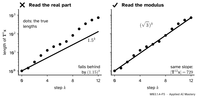
M03.1.4-F5
Wrong beside right. The real part \(\frac32\) underestimates the growth; the modulus \(\sqrt3\) gets it, up to a bounded wobble caused by the skewed basis.
“Complex eigenvalues are a rounding artefact; keep the real part.”
They are exact: \({\lambda^2 - 3\lambda + 3}\) has no real root. The real part alone predicts growth by \(1.5\) per step, but \(\mat{T}^{12}\) multiplies by \(729 = {(\sqrt3)^{12}}\), not by \({1.5^{12} \approx 130}\). Growth is read from the modulus.
“\(\mat{T}\) turns every vector by \(30^\circ\).”
Only in the coordinates of \(\vect{c}_1, \vect{c}_2\). In the standard picture \(\mat{T}\) turns \(\ihat\) to \((1, -1)\), a turn of \(45^\circ\), and \(\jhat\) to \((1, 2)\), a turn of about \(26.6^\circ\). What is exactly \(30^\circ\) is the average: twelve applications make one full turn.
“A spectral radius below 1 means every step shrinks every vector.”
It means that vectors shrink in the long run. The skewed basis can make a vector grow for a few steps first, because \(\mat{C}\) stretches some directions more than others: \(\mat{T}/1.8\) has \(\rho \approx 0.96\), yet it sends \((0, 1)\) to a vector of length about 1.24. In a recurrent network that transient growth is real, which is one reason why later courses look at the singular values of the weight matrix as well as its eigenvalues (M03.5).
Frontier note: eigenvalues and the training of recurrent networks
Pascanu, Mikolov and Bengio analysed a linear recurrent network, where the gradient flowing back through \(t\) steps is multiplied by the recurrent weight matrix \(t\) times. They showed that a largest eigenvalue modulus below 1 is sufficient for the long-term gradient components to vanish, and one above 1 is necessary for them to explode (Section 2.1). Against explosion they rescale the gradient whenever its norm passes a threshold (Section 3.2). Against vanishing they add a regularisation term that prefers weights for which the error signal keeps its norm as it travels back in time (Section 3.3). Both remedies act on the very quantity this lesson computes: how much repeated multiplication by one matrix stretches or shrinks a vector.
Check yourself
Recall
1. What are the eigenvalues of the rotation \(\mat{R}(\theta)\), and why is neither real when \(\theta\) is not a multiple of \(180^\circ\)?
Show answer
\(e^{\pm i\theta} = {\cos\theta \pm i\sin\theta}\). The discriminant \({-4\sin^2\theta}\) is negative unless \(\sin\theta = 0\).
2. Why do the complex eigenvalues of a real matrix come in conjugate pairs?
Show answer
Conjugating \({\mat{A}\vect{v}} = {\lambda\vect{v}}\) leaves the real \(\mat{A}\) unchanged and gives \({\mat{A}\vect{v}^*} = {\lambda^*\vect{v}^*}\).
3. What are the modulus and argument of the eigenvalues of \(\mat{T}\), and what do they mean?
Show answer
Modulus \(\sqrt3\), the stretch per step; arguments \(\pm 30^\circ\), the turn per step in the basis \(\vect{c}_1, \vect{c}_2\).
4. How is the basis \(\vect{c}_1, \vect{c}_2\) built from a complex eigenvector?
Show answer
Write the eigenvector as \({\vect{c}_1 + i\,\vect{c}_2}\) with real \(\vect{c}_1, \vect{c}_2\): they are its real and imaginary parts.
5. What is the spectral radius, and what does it predict?
Show answer
The largest modulus of an eigenvalue. Below 1, repeated application shrinks every vector in the long run; above 1, it makes some vectors grow without bound.
Exercises
1.★ Find the eigenvalues of the quarter turn \(\begin{bmatrix} 0 & -1 \\ 1 & 0 \end{bmatrix}\) from its characteristic polynomial, with their moduli and arguments.
Show solution
Trace 0 and determinant 1 give \({\lambda^2 + 1} = 0\), so \(\lambda = \pm i\). Both have modulus 1 and arguments \(\pm 90^\circ\), as Step 1 predicts with \(\theta = 90^\circ\).
2.★★ For \(\mat{M} = \begin{bmatrix} 1 & -1 \\ 1 & 1 \end{bmatrix}\), find the eigenvalues, the spectral radius and \(\mat{M}^8\).
Show solution
Trace 2 and determinant \({1 + 1} = 2\) give \({\lambda^2 - 2\lambda + 2} = 0\), so \({\lambda = 1 \pm i}\), with modulus \(\sqrt2\) and argument \(\pm 45^\circ\); \(\rho(\mat{M}) = \sqrt2\). \(\mat{M}\) is already \(\sqrt2\) times the anticlockwise turn by \(45^\circ\), because its columns are \({\sqrt2\,(\cos 45^\circ, \sin 45^\circ)}\) and \({\sqrt2\,(-\sin 45^\circ, \cos 45^\circ)}\). Eight turns of \(45^\circ\) are a full turn, so \({\mat{M}^8} = {(\sqrt2)^8\,\mat{I}} = {16\,\mat{I}}\).
3.★★★ Use \({\mat{T}^k} = {\mat{C}\,(\sqrt3)^k\mat{R}(-30k^\circ)\,\mat{C}^{-1}}\) to show that \({\mat{T}^6} = {-27\,\mat{I}}\), and confirm it by computing \(\mat{T}^2\), \(\mat{T}^3\) and then \({\mat{T}^6} = {(\mat{T}^3)^2}\).
Show solution
With \(k = 6\): \({(\sqrt3)^6} = 27\) and \({\mat{R}(-180^\circ)} = -\mat{I}\), so \({\mat{T}^6} = {\mat{C}\,(-27\,\mat{I})\,\mat{C}^{-1}} = {-27\,\mat{C}\mat{C}^{-1}} = {-27\,\mat{I}}\).
Sources. Each was opened and checked against this lesson on 15 November 2026.
Dan Margalit and Joseph Rabinoff, Interactive Linear Algebra, Section 5.5, Complex eigenvalues (open textbook, Georgia Tech). The rotation-scaling theorem: with \({C = [\operatorname{Re}v \;\; \operatorname{Im}v]}\), \({A = CBC^{-1}}\) where \(B\) has rows \({(\operatorname{Re}\lambda, \operatorname{Im}\lambda)}\) and \({(-\operatorname{Im}\lambda, \operatorname{Re}\lambda)}\), the form used here with \({\lambda = a + bi}\); complex eigenvalues of real matrices come in conjugate pairs; vectors spiral out when \({\abs{\lambda} > 1}\), in when \({\abs{\lambda} < 1}\), and go round an ellipse when \({\abs{\lambda} = 1}\).
Gilbert Strang, Eigenvalues and eigenvectors, MIT OpenCourseWare 18.06SC, lecture 21, and its lecture summary. The 90-degree rotation has trace 0, determinant 1 and eigenvalues \(i\) and \(-i\); if \({a + bi}\) is an eigenvalue of a real matrix, so is \({a - bi}\).
Sheldon Axler, Linear Algebra Done Right, 4th edition (open access). Example 5.9: the 90-degree rotation has no eigenvalues over the real numbers and the eigenvalues \(i\) and \(-i\) over the complex numbers.
Razvan Pascanu, Tomas Mikolov and Yoshua Bengio, On the difficulty of training recurrent neural networks, arXiv 1211.5063, Section 2.1. For a linear recurrent model, a largest eigenvalue below 1 in absolute value is sufficient for long-term gradient components to vanish, and one above 1 is necessary for them to explode; Sections 3.2 and 3.3 give gradient-norm clipping and a regulariser that keeps the back-propagated error’s norm.
NumPy reference, numpy.linalg.eig and numpy.angle. For a real matrix, eig returns real eigenvalues or conjugate pairs; angle returns the argument of a complex number, in radians unless deg=True.
Next. Module M03.2, Diagonalization and matrix powers, puts \(n\) independent eigenvectors into a matrix and computes \({\mat{A}^k}\) the easy way.