Some bases make a map look simple. Find the basis in which a map of the plane is nothing but a stretch along two directions, watch its matrix turn diagonal, and see how the same move gives fast powers, eigenvectors and principal component analysis.
Read a diagonal matrix as a map that stretches along each basis direction without mixing them.
Find the directions that a given 2 by 2 map leaves on their own lines, and the stretch factor along each.
Change to the basis of those directions and verify by hand that the matrix becomes diagonal.
Use the diagonal form to compute a power of a matrix.
Explain why some maps have no such basis, and what principal component analysis has to do with one.
In review. The maths and code on this page are checked by automated tests on every change, but an independent reader has not signed it off yet. Spot a mistake or a confusing step? Tell us.
The question
The last lesson showed that one map has a different matrix in each basis. Then some bases must be better than others. Is there a basis in which a map is as simple as a map can be: a stretch along one direction, a stretch along another, and nothing else? Finding that basis is what principal component analysis does to a data set, and it is the idea at the heart of the next course.
From the last lesson
1. State the rule for the matrix of a map in a new basis, and say what each of the three matrices does.
Show answer
\(\mat{A}_B = \mat{P}^{-1}\mat{A}\mat{P}\). Reading from the right: \(\mat{P}\) translates the input into standard coordinates, \(\mat{A}\) applies the map, and \(\mat{P}^{-1}\) translates the image back.
2. Name two numbers that similar matrices always share.
Show answer
The determinant and the trace.
Intuition
The simplest matrices are diagonal: zero everywhere except on the diagonal. The matrix with diagonal entries 3 and 1 sends \((c_1, c_2)\) to \((3c_1, c_2)\). Each coordinate is scaled on its own and neither leaks into the other. In pictures, each basis vector is stretched along its own line and is not turned.
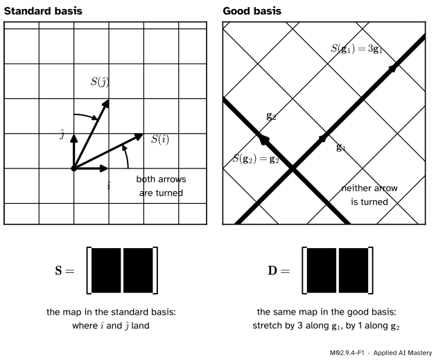
Most maps do not look like that. Take the map \(S(x, y) = {(2x + y,\; x + 2y)}\), with matrix \(\mat{S} = \begin{bmatrix} 2 & 1 \\ 1 & 2 \end{bmatrix}\). It turns both \(\ihat\) and \(\jhat\). But try the two arrows \(\vect{g}_1 = (1, 1)\) and \(\vect{g}_2 = (-1, 1)\):
Neither is turned. One is stretched by 3 and the other is left alone.
M02.9.4-F1
The same map \(S\) in two bases. In the standard basis both basis vectors are turned, and the matrix is full. In the basis \(\vect{g}_1, \vect{g}_2\) each basis vector stays on its own line, and the matrix is diagonal.
In the basis \(\vect{g}_1, \vect{g}_2\) the record of \(S\) is as short as a record can be: “stretch by 3 along the first, by 1 along the second”. A good basis for a map is one that makes its matrix diagonal.
Build it up
Step 1. Diagonal means no mixing. For \(\mat{D} = \begin{bmatrix} d_1 & 0 \\ 0 & d_2 \end{bmatrix}\) the row rule gives \(\mat{D}\,(c_1, c_2) = {(d_1c_1 + 0 \cdot c_2,\; 0 \cdot c_1 + d_2c_2)} = {(d_1c_1,\; d_2c_2)}\).
Step 2. What a good basis vector must do. Column \(j\) of the matrix in a new basis is where basis vector \(j\) lands, in the new coordinates (last lesson). For that column to be zero except in place \(j\), the image must be a multiple of the basis vector itself: \(S(\vect{g}) = k\,\vect{g}\). The vector may be stretched, shrunk or flipped, but it must stay on its own line.
Step 3. Hunt for such directions. We want \((x, y) \neq (0, 0)\) and a number \(k\) with \(S(x, y) = k\,(x, y)\), that is, \(2x + y = kx\) and \(x + 2y = ky\). Add the two equations, then subtract the second from the first:
\[
\begin{aligned}
3\,(x + y) &= k\,(x + y), \\
x - y &= k\,(x - y) .
\end{aligned}
\]
Rearranged, \({(k - 3)}{(x + y)} = 0\) and \({(k - 1)}{(x - y)} = 0\). If \(k\) is neither 3 nor 1, then \(x + y = 0\) and \(x - y = 0\), which forces \(x = y = 0\). So only two factors are possible.
\(k = 3\): the second equation becomes \(2\,{(x - y)} = 0\), so \(y = x\). That is the line of \(\vect{g}_1 = (1, 1)\).
\(k = 1\): the first equation becomes \(-2\,{(x + y)} = 0\), so \(y = -x\). That is the line of \(\vect{g}_2 = (-1, 1)\).
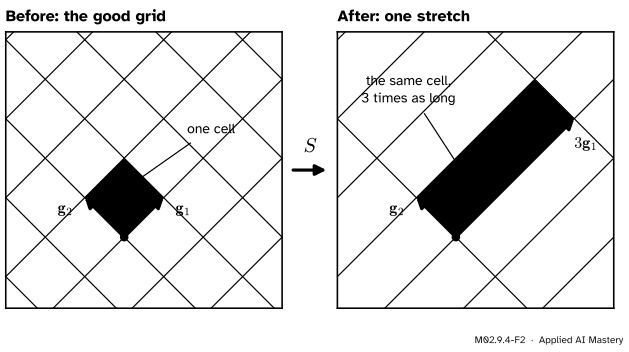
Step 4. See the map on its good grid.
M02.9.4-F2
On the grid of its good basis, \(S\) is a single stretch: three times as long along \(\vect{g}_1\), unchanged along \(\vect{g}_2\). No grid line is turned.
Step 5. Why it is worth the trouble. In the good basis, applying the map twice multiplies each coordinate twice: \((c_1, c_2)\) goes to \({(3^2c_1,\; 1^2c_2)}\). Applying it a hundred times is no harder. Powers of a full matrix are hard work. Powers of a diagonal one are free.
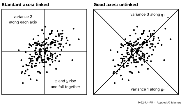
Step 6. The same move on data: a first look at PCA. A cloud of data points has a covariance matrix. Its diagonal holds the variance of each coordinate, which measures how spread out that coordinate is. Its other entries measure how strongly two coordinates rise and fall together.
M02.9.4-F5
A cloud whose covariance matrix is exactly \(\mat{S}\). On the standard axes the two coordinates are linked. On the axes of the good basis they are not, and the variances 3 and 1 can be read off separately.
Rewrite every point in the good basis of \(\mat{S}\), with the basis vectors scaled to length 1, and the covariance matrix becomes \(\mat{D}\). That is principal component analysis: choose the basis in which the covariance matrix is diagonal. The direction with the largest variance is the first principal component.
The formal statement
NoteResult: a basis of kept directions makes the matrix diagonal
Let \(\mat{A}\) be an \({n \times n}\) matrix and let \(\vect{g}_1, \dots, \vect{g}_n\) be a basis of \(\R^n\) with change-of-basis matrix \(\mat{P}\). Then
Proof. Call the basis \(G\) and write \(\vect{e}_j\) for the list with 1 in place \(j\) and 0 elsewhere.
If each basis vector is kept on its line. Column \(j\) of \(\mat{P}^{-1}\mat{A}\mat{P}\) is \([\mat{A}\vect{g}_j]_G\) (last lesson). Using \(\mat{A}\vect{g}_j = k_j\vect{g}_j\), then the fact that coordinates respect scaling (lesson M02.9.1), then \([\vect{g}_j]_G = \vect{e}_j\):
So column \(j\) has \(k_j\) in place \(j\) and zeros elsewhere. The matrix is diagonal.
If the matrix is diagonal. Call it \(\mat{D}\). Multiply \(\mat{P}^{-1}\mat{A}\mat{P} = \mat{D}\) on the left by \(\mat{P}\) to get \(\mat{A}\mat{P} = \mat{P}\mat{D}\). Column \(j\) of the left side is \(\mat{A}\vect{g}_j\). Column \(j\) of the right side is \(\mat{P}\) applied to column \(j\) of \(\mat{D}\), which is \(\mat{P}(k_j\vect{e}_j) = k_j\vect{g}_j\). So \(\mat{A}\vect{g}_j = k_j\vect{g}_j\). \(\blacksquare\)
A non-zero vector that a map keeps on its own line is called an eigenvector of the map, and its stretch factor is the eigenvalue. Course M03 is about finding them. In those words the result says: a good basis is a basis of eigenvectors.
Powers. Multiply \(\mat{D} = \mat{P}^{-1}\mat{A}\mat{P}\) on the left by \(\mat{P}\) and on the right by \(\mat{P}^{-1}\):
Then \(\mat{A}^2 = \mat{P}\mat{D}\,(\mat{P}^{-1}\mat{P})\,\mat{D}\mat{P}^{-1} = \mat{P}\mat{D}^2\mat{P}^{-1}\), and repeating the step, \(\cmodel{\mat{A}^m} = \mat{P}\,\cgrad{\mat{D}^m}\,\mat{P}^{-1}\) for every whole number \(m \ge 1\). The hard power is traded for an easy one, because \(\mat{D}^m\) just raises each diagonal entry to the power \(m\).
Not every map has a good basis. The course’s running map \(T(x, y) = {(x + y,\; -x + 2y)}\) keeps no direction on its line (exercise 3), so no basis makes it diagonal. But every symmetric matrix, one that equals its own transpose like \(\mat{S}\), does have a good basis, and its vectors can be chosen perpendicular. Every covariance matrix is symmetric, which is why PCA always works.
Go deeper: why PCA insists on perpendicular basis vectors of length 1
A map and a covariance matrix change differently under a new basis. Let the data points be \(\vect{x}_1, \dots, \vect{x}_N\) with mean zero, so that their covariance matrix is \(\mat{C} = \frac{1}{N-1}\sum_i \vect{x}_i\vect{x}_i\T\). The new coordinates of each point are \(\vect{z}_i = \mat{P}^{-1}\vect{x}_i\), which also have mean zero. Transposing a matrix times a vector reverses the order, \((\mat{M}\vect{x})\T = \vect{x}\T\mat{M}\T\), because entry \(j\) of each side is \(\sum_k m_{jk}\,x_k\). So
Add these up over the points and divide by \(N - 1\). The two outer matrices are the same in every term, so the covariance matrix of the new coordinates is
That is not \(\mat{P}^{-1}\mat{C}\mat{P}\) in general. The two agree whenever \((\mat{P}^{-1})\T = \mat{P}\), that is, when the inverse of \(\mat{P}\) is its transpose. Lesson M02.10.2 shows that this happens exactly when the columns of \(\mat{P}\) are perpendicular and of length 1. With such a basis the covariance matrix changes the way a map does, and the good basis of \(\mat{C}\) makes it diagonal.
Worked example
Change \(\mat{S} = \begin{bmatrix} 2 & 1 \\ 1 & 2 \end{bmatrix}\) to its good basis \(\vect{g}_1 = (1, 1)\), \(\vect{g}_2 = (-1, 1)\), then use the result.
The change-of-basis matrix and its inverse.\(\mat{P} = \begin{bmatrix} 1 & -1 \\ 1 & 1 \end{bmatrix}\) has \({ps - qr} = {1 \cdot 1} - {(-1) \cdot 1} = 2\), so \(\mat{P}^{-1} = \tfrac12\begin{bmatrix} 1 & 1 \\ -1 & 1 \end{bmatrix}\).
Check with the last lesson. The trace is \(3 + 1 = 4 = 2 + 2\) and the determinant is \({3 \cdot 1} = 3 = {2 \cdot 2} - {1 \cdot 1}\). Both survived, as they must.
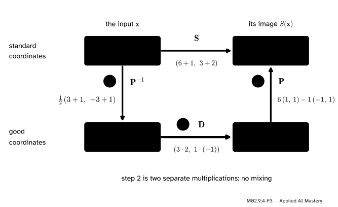
Apply \(S\) to \(\vect{x} = (3, 1)\) by way of the good basis.
M02.9.4-F3
The map applied the long way round. Translate into the good basis, scale each coordinate on its own, and translate back. The answer matches the direct product.
A power. To apply \(S\) five times, use \(\mat{S}^5 = \mat{P}\mat{D}^5\mat{P}^{-1}\) with \(3^5 = 243\) and \(1^5 = 1\). First \(\mat{P}\mat{D}^5\), then that product times \(\mat{P}^{-1}\):
NumPy can find the good directions itself. For a symmetric matrix, np.linalg.eigh returns the stretch factors in increasing order and the kept directions as columns, scaled to length 1. For any square matrix, np.linalg.eig does the same job, in no promised order.
import numpy as npS = np.array([[2.0, 1.0], [1.0, 2.0]])P = np.array([[1.0, -1.0], [1.0, 1.0]])print("P^-1 S P =\n", np.linalg.solve(P, S @ P))print("S^5 =\n", np.linalg.matrix_power(S, 5))factors, directions = np.linalg.eigh(S) # S is symmetricprint("stretch factors:", factors.round(6))print("kept directions (columns):\n", directions.round(4))T = np.array([[1.0, 1.0], [-1.0, 2.0]]) # the course's running mapprint("stretch factors of T:", np.linalg.eig(T)[0].round(4))
For \(T\) the answer contains \(j\), Python’s sign for the square root of \(-1\). That is NumPy’s way of saying that no real direction stays on its line.
Last, the data cloud of the figure. It is built in the good basis first, with variances 3 and 1 and no link, and then translated into standard coordinates with \(\mat{P}\).
from sklearn.decomposition import PCArng = np.random.default_rng(7)n =200a = rng.normal(size=n); a -= a.mean()b = rng.normal(size=n); b -= b.mean()b -= (a @ b) / (a @ a) * a # remove the part of b that lies along a# Coordinates in the good basis: variance 3, variance 1, and no link.Z = np.column_stack([np.sqrt(3) * a / a.std(ddof=1), b / b.std(ddof=1)])Q = P / np.sqrt(2) # the good basis, scaled to length 1X = Z @ Q.T # rows x = Q z: good -> standardprint("covariance, standard axes:\n", np.cov(X, rowvar=False).round(6))back = np.linalg.solve(Q, X.T).T # rows z = Q^-1 x: standard -> goodprint("covariance, good axes:\n", np.cov(back, rowvar=False).round(6) +0.0) # + 0.0 shows -0.0 as 0.0pca = PCA(n_components=2).fit(X)variances = pca.explained_variance_print("PCA variances: ", variances.round(6))print("PCA directions:\n", pca.components_.round(4))
scikit-learn’s PCA, handed only the points, recovers the variances 3 and 1 and the two good directions (up to sign). It found the basis in which the cloud is simplest.
Explore
This module’s interactive, the two-grid viewer, lives in lesson M02.9.2. Set its basis to \(\vect{g}_1 = (1, 1)\) and \(\vect{g}_2 = (-1, 1)\) with the sliders. Put the arrow at \((2, 0)\) and read its good coordinates, \((1, -1)\). Then put it at \((4, 2)\), which is \(S(2, 0)\), and read \((3, -1)\): the first coordinate tripled and the second did not change.
Pitfalls
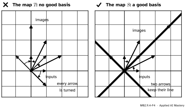
M02.9.4-F4
Wrong beside right. The running map \(T\) turns every arrow, so no basis can make it diagonal. The map \(S\) keeps two lines, and those two lines give its good basis.
“Every matrix becomes diagonal if you pick the right basis.”
A good basis needs enough directions that the map keeps on their lines. The running map \(T\) keeps none (exercise 3). The shear \(\begin{bmatrix} 1 & 1 \\ 0 & 1 \end{bmatrix}\) keeps only one, the horizontal line, and one direction is not a basis of the plane. Symmetric matrices are the safe case, and covariance matrices are symmetric.
“A good basis is good for every map.”
A basis is good for a map. In the basis \(\vect{g}_1, \vect{g}_2\) the matrix of \(S\) is diagonal, but the matrix of \(T\) is \(\tfrac12\begin{bmatrix} 3 & 3 \\ -1 & 3 \end{bmatrix}\), as full as ever. The same holds for data: the basis that PCA finds belongs to one data set. A different data set has its own.
“The diagonal entries say how much the map stretches along the \(x\) and \(y\) axes.”
They say how much it stretches along \(\vect{g}_1\) and \(\vect{g}_2\). A diagonal matrix must be read in its own basis. \(S\) stretches by 3 along the diagonal line \(y = x\), and it does not stretch anything by 3 along the \(x\) axis: \(S(1, 0) = (2, 1)\).
Check yourself
Recall
1. What does a diagonal matrix do to a list of coordinates?
Show answer
It multiplies each coordinate by its own diagonal entry and never mixes them: \((c_1, c_2)\) goes to \((d_1c_1, d_2c_2)\).
2. What must a map do to a basis vector for the matrix in that basis to be diagonal?
Show answer
Keep it on its own line: send it to a multiple of itself, \(\mat{A}\vect{g} = k\,\vect{g}\).
3. What are the good basis and the diagonal matrix for \(\mat{S} = \begin{bmatrix} 2 & 1 \\ 1 & 2 \end{bmatrix}\)?
Show answer
\(\vect{g}_1 = (1, 1)\) with factor 3 and \(\vect{g}_2 = (-1, 1)\) with factor 1, so the diagonal entries are 3 and 1.
4. How does a good basis make the power \(\mat{A}^m\) easy?
Show answer
\(\mat{A}^m = \mat{P}\mat{D}^m\mat{P}^{-1}\), and \(\mat{D}^m\) only needs each diagonal entry raised to the power \(m\).
5. In one sentence, what does principal component analysis choose?
Show answer
The basis of perpendicular unit vectors in which the covariance matrix of the data is diagonal, so that the new coordinates are no longer linked.
Exercises
1.★ Use the three-step route through the good basis to compute \(S(1, 3)\), and check the answer directly.
2.★★ For \(\mat{M} = \begin{bmatrix} 1 & 2 \\ 2 & 1 \end{bmatrix}\), find the directions that the map keeps on their lines and their factors, by adding and subtracting the two equations as in Step 3. Write the diagonal matrix, and use it to find \(\mat{M}^4\).
Show solution
We need \(x + 2y = kx\) and \(2x + y = ky\). Adding gives \(3\,{(x + y)} = k\,{(x + y)}\). Subtracting the second from the first gives \(-{(x - y)} = k\,{(x - y)}\). So \({(k - 3)}{(x + y)} = 0\) and \({(k + 1)}{(x - y)} = 0\).
If \(k = 3\), the second equation gives \(x = y\): the direction \((1, 1)\). If \(k = -1\), the first gives \(y = -x\): the direction \((-1, 1)\). Any other \(k\) forces \(x = y = 0\). So in the basis \((1, 1), (-1, 1)\) the matrix is diagonal with entries \(3\) and \(-1\). The factor \(-1\) means that direction is flipped.
The basis is the one from the lesson, so \(\mat{P}\) and \(\mat{P}^{-1}\) are the same. Call the diagonal matrix \(\mat{D}\). With \(3^4 = 81\) and \((-1)^4 = 1\), \(\mat{M}^4 = \mat{P}\mat{D}^4\mat{P}^{-1}\):
Check: \(\mat{M}^2 = \begin{bmatrix} 5 & 4 \\ 4 & 5 \end{bmatrix}\), and squaring that gives \(\begin{bmatrix} 25 + 16 & 20 + 20 \\ 20 + 20 & 16 + 25 \end{bmatrix}\), the same matrix.
3.★★★ Show that the running map \(T(x, y) = {(x + y,\; -x + 2y)}\) keeps no direction on its own line: the only vector with \(T(x, y) = k\,(x, y)\) for some real number \(k\) is the zero vector.
Show solution
Suppose \(x + y = kx\) and \(-x + 2y = ky\). The first equation gives \(y = {(k - 1)}\,x\). Put that into the second, written as \(-x + {(2 - k)}\,y = 0\):
\[
-x + (2 - k)(k - 1)\,x = 0 .
\]
Expand \({(2 - k)}{(k - 1)} = -k^2 + 3k - 2\), so the equation is \({(-k^2 + 3k - 3)}\,x = 0\), that is,
\[
(k^2 - 3k + 3)\,x = 0 .
\]
Complete the square: \(k^2 - 3k + 3 = {(k - \tfrac32)^2} + \tfrac34\), which is at least \(\tfrac34\) for every real \(k\) and so is never zero. Therefore \(x = 0\), and then \(y = {{(k - 1)} \cdot 0} = 0\). Only the zero vector is “kept”, and the zero vector is not a direction. So \(T\) has no good basis of real vectors, which is what the figure in the pitfalls shows.
Summary card
A good basis turns a map into separate stretches, and its matrix into a diagonal one.
M02.9.4-F1
Kept directions make it diagonal.
Diagonal.\(\mat{D}\,(c_1, c_2) = {(d_1c_1,\; d_2c_2)}\): no mixing.
Good basis.\(\mat{P}^{-1}\mat{A}\mat{P}\) is diagonal exactly when \(\mat{A}\vect{g}_j = k_j\vect{g}_j\) for each basis vector.
This lesson’s example.\(\mat{S} = \begin{bmatrix} 2 & 1 \\ 1 & 2 \end{bmatrix}\) keeps \((1, 1)\) with factor 3 and \((-1, 1)\) with factor 1.
Not always possible. Some maps, such as the running map \(T\), keep no direction.
Sources and next steps
Sources. Each was opened and checked against this lesson on 12 November 2026.
Dan Margalit and Joseph Rabinoff, Interactive Linear Algebra, Section 5.4, Diagonalization (open textbook, Georgia Tech). The diagonalization theorem: a matrix is similar to a diagonal one exactly when it has \(n\) independent eigenvectors, which then form the columns of the change-of-basis matrix. It also gives \(A^n = CD^nC^{-1}\) and the shear as a matrix that cannot be made diagonal.
Grant Sanderson, Eigenvectors and eigenvalues, 3Blue1Brown, Linear Algebra, chapter 14. Eigenvectors as vectors that remain on their own span, the rotation and the shear as maps with too few of them, and the advice to change to an eigenbasis to compute a high power.
Sheldon Axler, Linear Algebra Done Right, 4th edition (open access). Definition 5.50 and result 5.55: an operator has a diagonal matrix in some basis exactly when the space has a basis of eigenvectors. Result 7.29, the real spectral theorem, says that a self-adjoint operator has a diagonal matrix in some orthonormal basis. On \(\R^n\) with the dot product, a map is self-adjoint exactly when its matrix is symmetric, so a symmetric matrix has a good basis of perpendicular unit vectors.
Gilbert Strang, Change of basis; image compression, MIT OpenCourseWare 18.06SC, lecture 31. The lecture summary notes that in a basis of eigenvectors the matrix of a transformation is the diagonal matrix of eigenvalues.
scikit-learn reference, sklearn.decomposition.PCA. components_ holds the principal axes, the directions of maximum variance, and explained_variance_ equals the largest eigenvalues of the covariance matrix of the data.
NumPy reference, numpy.linalg.eigh, numpy.linalg.eig, numpy.linalg.matrix_power and numpy.cov. eigh takes a symmetric matrix and returns its eigenvalues in ascending order with normalised eigenvectors as columns. eig returns complex eigenvalues in conjugate pairs for a real matrix that has no real ones.
Next. Module M02.10, Orthogonality, Gram-Schmidt and QR, studies the bases that are easiest to work with: perpendicular unit vectors, for which the inverse of \(\mat{P}\) is simply its transpose. Course M03 then finds good bases for general matrices.