A matrix need not be square. An m-by-n matrix takes n numbers in and gives m out: one column per input direction, each with m entries. See a 2-by-3 matrix squash space onto a plane, a 3-by-2 matrix place a plane inside space, and why a neural-network layer’s weights have the shape (outputs, inputs).
Read the shape of a matrix: say how many numbers it takes in, how many it gives out, and when a product with a vector is defined.
Compute the product of a matrix of any shape with a vector, by columns and by rows.
Describe in pictures what a wide matrix loses and what a tall matrix cannot reach.
Explain why a layer with n inputs and m outputs has a weight matrix of shape (m, n), and tell a matrix that is a map from one that is a table of data.
In review. The maths and code on this page are checked by automated tests on every change, but an independent reader has not signed it off yet. Spot a mistake or a confusing step? Tell us.
The question
A drawing of a cube on flat paper turns three coordinates into two. One layer of a neural network may take in the 784 pixels of a small image and give out 10 scores. Neither can be a square matrix. What does a matrix do when its output has a different number of dimensions from its input, and what is lost, or left empty, when it does?
From the last lesson
1. Write the matrix of a rotation by the angle \(\theta\).
Show answer
\(\begin{bmatrix} \cos\theta & -\sin\theta \\ \sin\theta & \cos\theta \end{bmatrix}\). Its columns are \((\cos\theta, \sin\theta)\) and \((-\sin\theta, \cos\theta)\).
2. In which direction does a positive angle turn the plane?
Show answer
Anticlockwise, the direction in which angles are measured on the unit circle.
Intuition
“The columns are where the basis vectors land.” Nothing in that sentence says the landing spots must live in the same space the basis vectors came from.
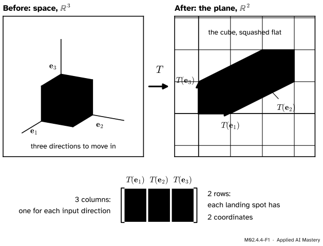
Space, \(\R^3\), has three basis vectors: \(\vect{e}_1 = (1, 0, 0)\), \(\vect{e}_2 = (0, 1, 0)\) and \(\vect{e}_3 = (0, 0, 1)\). A linear map from space to the plane must send each of them to a point of the plane, and a point of the plane has two coordinates. Three landing spots, two numbers each: that is a matrix with three columns and two rows.
M02.4.4-F1
A \(2 \times 3\) matrix is a map from space to the plane. Its three columns are where the three basis vectors of space land, and each landing spot has two coordinates. The cube on the left is squashed flat on the right.
The picture on the right is flat, although your eye may insist on seeing a box. Every drawing of a box in which parallel edges stay parallel can be made by a \(2 \times 3\) matrix.
Build it up
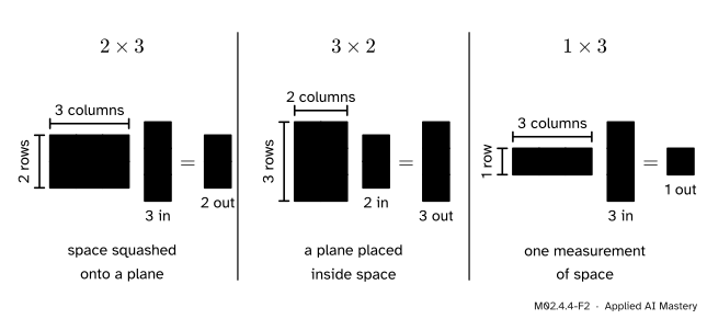
Step 1. Read the shape. A matrix with \(m\) rows and \(n\) columns is called \(m \times n\), rows first. Its \(n\) columns are the landing spots of \(n\) basis vectors, so the input has \(n\) coordinates. Each column has \(m\) entries, so the output has \(m\) coordinates.
M02.4.4-F2
The shape of a matrix is “outputs by inputs”. The number of columns is the number of entries the input must have. The number of rows is the number of entries the output will have.
So an \(m \times n\) matrix is a map from \(\R^n\) to \(\R^m\). Notice the order: the second number is the size of the input.
Step 2. A wide matrix squashes. Take the matrix of the anchor figure,
Its three columns, \(\vect{a}_1 = (1, 0)\), \(\vect{a}_2 = (2, 1)\) and \(\vect{a}_3 = (0, 1)\), are three arrows in a plane, and a plane has room for only two independent directions (M02.2). So one arrow must be a combination of the other two. Here \(\vect{a}_2 = 2\vect{a}_1 + \vect{a}_3\), since \(2\,(1, 0) + (0, 1) = (2, 1)\). So one step of \(\vect{e}_2\) lands in exactly the same place as two steps of \(\vect{e}_1\) and one of \(\vect{e}_3\). Different inputs, same output: the map cannot be undone.
Step 3. A tall matrix cannot fill its target. Now go the other way, from the plane into space:
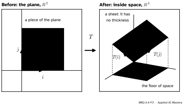
Its columns say that \(T(\ihat) = (1, 0, 1)\) and \(T(\jhat) = (0, 1, 1)\): two points of space.
M02.4.4-F3
A \(3 \times 2\) matrix places the plane inside space. The grid arrives undamaged, as a tilted sheet through the origin. Most of space is not on the sheet, so most of space is never reached.
Every output is \(x\,(1, 0, 1) + y\,(0, 1, 1) = (x, y, x + y)\). The third coordinate is always the sum of the first two. A point such as \((0, 0, 1)\) breaks that rule, so no input lands on it.
Step 4. One row is one measurement. The extreme case is a matrix with a single row, such as \(\begin{bmatrix} 1 & 2 & 0 \end{bmatrix}\). It is \(1 \times 3\): three numbers in, one number out. Its three columns are the single numbers 1, 2 and 0, and
That is the dot product of M02.3. A \(1 \times n\) matrix measures its input and reports one number.
Step 5. Every matrix is a stack of measurements. The row we just used is the top row of \(\mat{A}\). By the row view of M02.4.2, the top entry of \(\mat{A}\vect{x}\) is that row times \(\vect{x}\), and the bottom entry is the bottom row times \(\vect{x}\). An \(m \times n\) matrix takes \(m\) measurements of the same input, one for each row.
This is exactly a layer of a neural network. Each output unit owns one row of weights and reports one measurement of the input. So a layer with \(n\) inputs and \(m\) outputs has a weight matrix of shape (outputs, inputs), \(m \times n\). The layer in the opening question has a \(10 \times 784\) matrix, which holds \(7{,}840\) weights.
The formal statement
NoteDefinition: the map of an \(m \times n\) matrix
Let \(\mat{A}\) have \(m\) rows and \(n\) columns, with columns \(\vect{a}_1, \dots, \vect{a}_n\) in \(\R^m\). For \(\vect{x} = (x_1, \dots, x_n)\) in \(\R^n\),
where \((\mat{A}\vect{x})_i\) is entry \(i\) of the result. The product is defined only when the number of columns of \(\mat{A}\) equals the number of entries of \(\vect{x}\). The result has as many entries as \(\mat{A}\) has rows.
The first formula is the column view: the columns weighted by the input’s coordinates. The second is the row view, row \(i\) times \(\vect{x}\). They agree as in M02.4.2, because entry \(i\) of the column \(\vect{a}_j\) is \(a_{ij}\).
M02.4.2 also showed that this map is linear, and that every linear map from \(\R^n\) to \(\R^m\) comes from exactly one \(m \times n\) matrix. What is new here is what the shape forces.
A lost direction means a whole line of inputs shares each output. Suppose some non-zero \(\vect{d}\) has \(\mat{A}\vect{d} = \vect{0}\). Then for any input \(\vect{x}\) and any number \(s\), linearity gives
The points \(\vect{x} + s\,\vect{d}\) form a line through \(\vect{x}\), and the whole line lands on the single point \(\mat{A}\vect{x}\). For our \(\mat{A}\) the direction is \(\vect{d} = (2, -1, 1)\): by Step 2, \(2\vect{a}_1 - \vect{a}_2 + \vect{a}_3 = \vect{0}\).
Two facts about every matrix of that shape.
If the matrix is wide (\(n > m\), more inputs than outputs), some non-zero input is always sent to zero, so the map always loses something.
If the matrix is tall (\(m > n\), more outputs than inputs), some point of \(\R^m\) is never an output, so the map can never fill its target.
We have checked both on our examples. The general proofs need the idea of dimension and come in M02.7. Axler states them as results 3.22 and 3.24.
Go deeper: a first look at null space and rank
The two things we have just met have names, which M02.7 studies properly. The null space of a matrix is the set of inputs it sends to zero. The column space is the set of all its outputs: every combination of its columns. The rank is the dimension of the column space, the number of independent directions the outputs can move in.
One count ties them together: the rank plus the dimension of the null space equals \(n\), the number of columns. Every input direction is either kept or lost. Check it on this lesson’s matrices.
\(\mat{A}\), \(2 \times 3\): the outputs fill the plane (rank 2) and one line is sent to zero (dimension 1). \(2 + 1 = 3\).
\(\mat{B}\), \(3 \times 2\): the outputs fill a sheet (rank 2) and only the origin is sent to zero (dimension 0). \(2 + 0 = 2\).
\(\begin{bmatrix} 1 & 2 & 0 \end{bmatrix}\), \(1 \times 3\): the outputs fill a number line (rank 1), and the inputs with \(x_1 + 2x_2 = 0\), a whole plane, are sent to zero (dimension 2). \(1 + 2 = 3\).
This is the fundamental theorem of linear maps (Axler, result 3.21).
Worked example
Compute \(\mat{A}\vect{x}\) for \(\mat{A} = \begin{bmatrix} 1 & 2 & 0 \\ 0 & 1 & 1 \end{bmatrix}\) and \(\vect{x} = (2, 1, 3)\). Then find other inputs with the same output.
Check the shapes first.\(\mat{A}\) is \(2 \times 3\) and \(\vect{x}\) has 3 entries, so the product is defined and has 2 entries.
Column view. Take 2 of the first column, 1 of the second and 3 of the third:
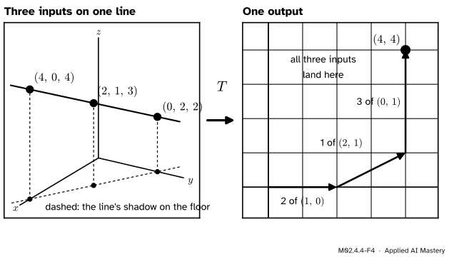
Other inputs with the same output. Step 2 found that one step of \(\vect{e}_2\) can be traded for two of \(\vect{e}_1\) and one of \(\vect{e}_3\) without moving the output. Make that trade in \(\vect{x} = (2, 1, 3)\): take away 1 from the second entry, add 2 to the first and 1 to the third. The result is \((4, 0, 4)\), and indeed \(4\,(1, 0) + 0\,(2, 1) + 4\,(0, 1) = (4, 4)\). Trade in the other direction and you get \((0, 2, 2)\), with \(0\,(1, 0) + 2\,(2, 1) + 2\,(0, 1) = (4, 2) + (0, 2) = (4, 4)\).
M02.4.4-F4
The worked example. On the right, the input \((2, 1, 3)\) is turned into the output \((4, 4)\) one column at a time. On the left, that input sits on a line in space, and every point of the line lands on the same output.
The three inputs differ by multiples of \(\vect{d} = (2, -1, 1)\): \((4, 0, 4) = \vect{x} + \vect{d}\) and \((0, 2, 2) = \vect{x} - \vect{d}\). Every point \(\vect{x} + s\,\vect{d}\) of that line lands on \((4, 4)\). Three numbers went in, two came out, and one direction’s worth of information is gone.
Code
A product for a matrix of any shape, from scratch: the column view with two loops, plus the shape check from the definition.
def matvec(A, x):"""A times x for a matrix of any shape. A is a list of rows.""" m, n =len(A), len(A[0])iflen(x) != n:raiseValueError(f"expected {n} entries, got {len(x)}") result = [0] * mfor j inrange(n): # one column for each entry of the inputfor i inrange(m): # each column has m entries result[i] += x[j] * A[i][j]return resultA = [[1, 2, 0], [0, 1, 1]] # 2 x 3: space to planeB = [[1, 0], [0, 1], [1, 1]] # 3 x 2: plane into spacer = [[1, 2, 0]] # 1 x 3: one measurementprint("A (2, 1, 3) =", matvec(A, [2, 1, 3]))print("A (4, 0, 4) =", matvec(A, [4, 0, 4]), " A (0, 2, 2) =", matvec(A, [0, 2, 2]))print("A (2, -1, 1) =", matvec(A, [2, -1, 1]), " <- the lost direction")print("B (2, -1) =", matvec(B, [2, -1]))print("r (2, 1, 3) =", matvec(r, [2, 1, 3]))try: matvec(A, [2, 1])exceptValueErroras error:print("A (2, 1) : error:", error)
A (2, 1, 3)  = [4, 4]
A (4, 0, 4)  = [4, 4]   A (0, 2, 2) = [4, 4]
A (2, -1, 1) = [0, 0]   <- the lost direction
B (2, -1)    = [2, -1, 1]
r (2, 1, 3)  = [4]
A (2, 1)     : error: expected 3 entries, got 2
Now NumPy. The attribute .shape is the pair (rows, columns), which is (outputs, inputs).
import numpy as npA, B, r = np.array(A), np.array(B), np.array(r)for name, M in [("A", A), ("B", B), ("r", r)]: m, n = M.shapeprint(f"{name}.shape = {M.shape}: takes {n} numbers in, gives {m} out")x = np.array([2, 1, 3])print("A @ x =", A @ x, " with shape", (A @ x).shape)print("one row at a time:", A[0] @ x, "and", A[1] @ x)try: B @ x # 2 columns, but 3 entriesexceptValueError:print("B @ x raises ValueError: the shapes do not match")
A.shape = (2, 3): takes 3 numbers in, gives 2 out
B.shape = (3, 2): takes 2 numbers in, gives 3 out
r.shape = (1, 3): takes 3 numbers in, gives 1 out
A @ x = [4 4]  with shape (2,)
one row at a time: 4 and 4
B @ x raises ValueError: the shapes do not match
Last, a layer. Its weight matrix has shape (outputs, inputs). A batch of inputs is stored as a table with one input in each row, and that changes how the product is written.
rng = np.random.default_rng(0)W = rng.normal(size=(2, 3)) # a layer with 3 inputs and 2 outputsone = np.array([2.0, 1.0, 3.0]) # one input: 3 numbersbatch = rng.normal(size=(4, 3)) # a table of 4 inputs, one in each ROWprint("one input ->", (W @ one).shape)print("a batch ->", (batch @ W.T).shape, " (one output in each row)")print("row 0 of the batch result equals W @ batch[0]:", np.allclose((batch @ W.T)[0], W @ batch[0]))
one input  -> (2,)
a batch    -> (4, 2)  (one output in each row)
row 0 of the batch result equals W @ batch[0]: True
batch @ W.T applies the same map to every row of the table. This is why PyTorch documents its linear layer as \(\vect{y} = \vect{x}\mat{A}\T + \vect{b}\) while storing the weight \(\mat{A}\) with shape (outputs, inputs).
Explore
The matrix playground of this module is in lesson M02.4.2. It stays in the plane, but it can show what losing a direction looks like. Press Squash onto a line: the two columns lie along one line, the area factor is 0, and the whole plane lands on that line. Drag \(\vect{v}\) and find different inputs with the same \(T(\vect{v})\). They lie on a line, like the three inputs of the worked example.
Pitfalls
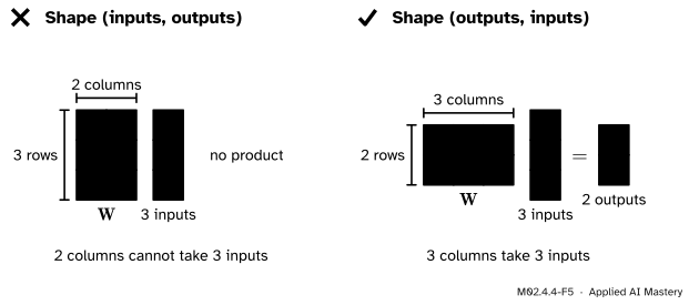
M02.4.4-F5
Wrong beside right, for a layer with 3 inputs and 2 outputs. The weight matrix needs one column for each input, so it is \(2 \times 3\), not \(3 \times 2\).
“An \(m \times n\) matrix takes \(m\) numbers in and gives \(n\) out.”
It is the other way round. The shape is rows by columns, and the columns match the input. A \(2 \times 3\) matrix takes 3 numbers in and gives 2 out. In code, a layer with 3 inputs and 2 outputs has W.shape == (2, 3). Build it as (3, 2) and W @ x fails, as the figure shows.
“A table of data and a weight matrix are the same kind of thing.”
Both are grids of numbers, and they mean different things. In a matrix used as a map, the columns are landing spots, and swapping two rows gives a different map. In a table of data, each row is one example and each column is one feature. Shuffling the rows leaves the dataset unchanged. A table of inputs goes through a layer as X @ W.T, one row at a time, not as W @ X.
“A \(2 \times 3\) matrix just drops the third coordinate.”
Only one very special matrix does that. In general a wide matrix loses a direction, which need not lie along an axis. Our \(\mat{A}\) loses \((2, -1, 1)\). It does not lose the third axis: \(\mat{A}\,\vect{e}_3 = (0, 1)\), which is not zero. The mirror-image mistake is to think a tall matrix creates information. Our \(\mat{B}\) gives three numbers, but the third is always the sum of the other two.
Check yourself
Recall
1. An \(m \times n\) matrix is a map from which space to which space?
Show answer
From \(\R^n\) to \(\R^m\). The number of columns is the size of the input, and the number of rows is the size of the output.
2. The matrix of a linear map from \(\R^3\) to \(\R^2\) has how many columns, with how many entries in each?
Show answer
Three columns, one for each basis vector of \(\R^3\), with two entries in each. It is \(2 \times 3\).
3. What does a \(1 \times n\) matrix do to a vector with \(n\) entries?
Show answer
It returns one number: the dot product of its single row with the vector.
4. When is the product \(\mat{A}\vect{x}\) defined?
Show answer
When the number of columns of \(\mat{A}\) equals the number of entries of \(\vect{x}\).
5. A neural-network layer has 5 inputs and 3 outputs. What is the shape of its weight matrix?
Show answer
\(3 \times 5\): shape (outputs, inputs). It holds 15 weights.
Exercises
1.★ A weight matrix \(\mat{W}\) has shape \((4, 7)\). (a) How many inputs and how many outputs does its layer have? (b) Is \(\mat{W}\vect{x}\) defined when \(\vect{x}\) has 7 entries? When it has 4? (c) How many weights does \(\mat{W}\) hold?
Show solution
(a) 7 inputs (columns) and 4 outputs (rows). (b) It is defined for 7 entries, and the result has 4 entries. It is not defined for 4 entries, because the matrix has 7 columns. (c) \(4 \times 7 = 28\).
2.★★ Let \(\mat{M} = \begin{bmatrix} 1 & 0 \\ 2 & 1 \\ 0 & 3 \end{bmatrix}\). (a) Compute \(\mat{M}\vect{v}\) for \(\vect{v} = (2, -1)\). (b) Is \((1, 0, 0)\) an output of this map?
Show solution
(a) \(\mat{M}\) is \(3 \times 2\) and \(\vect{v}\) has 2 entries, so the product is defined and has 3 entries. By columns, \(2\,(1, 2, 0) - 1\,(0, 1, 3) = (2, 4, 0) - (0, 1, 3) = (2, 3, -3)\).
(b) An output has the form \(x\,(1, 2, 0) + y\,(0, 1, 3) = (x,\; 2x + y,\; 3y)\). To equal \((1, 0, 0)\) we need \(x = 1\) from the first entry, then \(2 + y = 0\), so \(y = -2\), from the second. But then the third entry is \(3y = -6\), not 0. So \((1, 0, 0)\) is not an output. The outputs fill only a sheet inside space.
3.★★★ Let \(\mat{C} = \begin{bmatrix} 1 & 0 & -1 \\ 0 & 1 & 2 \end{bmatrix}\). (a) Find every \(\vect{x}\) with \(\mat{C}\vect{x} = \vect{0}\). (b) Show that two inputs \(\vect{u}\) and \(\vect{v}\) have the same output exactly when \(\vect{u} - \vect{v}\) is one of the vectors from (a).
Show solution
(a) By rows, \(\mat{C}\vect{x} = (x_1 - x_3,\; x_2 + 2x_3)\). Both entries are zero exactly when \(x_1 = x_3\) and \(x_2 = -2x_3\). Writing \(s\) for \(x_3\), the solutions are \(\vect{x} = s\,(1, -2, 1)\): a line through the origin. Check: \(1\,(1, 0) - 2\,(0, 1) + 1\,(-1, 2) = (0, 0)\).
(b) By linearity, \(\mat{C}(\vect{u} - \vect{v}) = \mat{C}\vect{u} - \mat{C}\vect{v}\). So \(\mat{C}\vect{u} = \mat{C}\vect{v}\) holds exactly when \(\mat{C}(\vect{u} - \vect{v}) = \vect{0}\), and by (a) that happens exactly when \(\vect{u} - \vect{v} = s\,(1, -2, 1)\) for some number \(s\). The inputs that share an output are the lines in the direction \((1, -2, 1)\).
Summary card
An \(m \times n\) matrix takes \(n\) numbers in and gives \(m\) out.
M02.4.4-F1
One column for each input direction.
Shape.\(m \times n\) means \(m\) rows and \(n\) columns, a map from \(\R^n\) to \(\R^m\): (outputs, inputs).
Product.\(\mat{A}\vect{x} = x_1\vect{a}_1 + \cdots + x_n\vect{a}_n\), defined when \(\mat{A}\) has as many columns as \(\vect{x}\) has entries.
Rows. Entry \(i\) of \(\mat{A}\vect{x}\) is row \(i\) times \(\vect{x}\): one measurement for each row.
Wide (\(n > m\)): a whole line of inputs shares each output. Something is lost.
Tall (\(m > n\)): the outputs form a sheet that cannot fill \(\R^m\).
In machine learning. A layer with \(n\) inputs and \(m\) outputs has weights of shape \((m, n)\).
Sources and next steps
Sources. Each was opened and checked against this lesson on 12 November 2026.
Sheldon Axler, Linear Algebra Done Right, 4th edition (open access). Section 3C: a linear map from an \(n\)-dimensional space to an \(m\)-dimensional space has an \(m\)-by-\(n\) matrix (3.31), with a \(3\)-by-\(2\) example (3.32). Section 3B: a linear map to a lower-dimensional space is not injective (3.22), a linear map to a higher-dimensional space is not surjective (3.24), and the fundamental theorem of linear maps (3.21).
Grant Sanderson, Nonsquare matrices as transformations between dimensions, 3Blue1Brown, Linear Algebra, chapter 8. The columns count the basis vectors of the input and the rows count the coordinates of each landing spot; a \(3 \times 2\) matrix sends the plane to a plane through the origin of space; a matrix with one row is tied to the dot product.
PyTorch documentation, torch.nn.Linear. The layer computes \(\vect{y} = \vect{x}\mat{A}\T + \vect{b}\), and its weight has shape (out_features, in_features).
NumPy manual, numpy.matmul. The @ operator is shorthand for np.matmul, and a ValueError is raised when the last dimension of the first argument does not match the second-to-last dimension of the second.
Next. One layer takes 784 numbers to 128, and the next takes those 128 to 10. Doing one map after another is multiplying their matrices: M02.5, Matrix multiplication as composition.