\( \newcommand{\vect}[1]{\mathbf{#1}} \newcommand{\mat}[1]{\mathbf{#1}} \newcommand{\R}{\mathbb{R}} \newcommand{\E}{\mathbb{E}} \newcommand{\Prob}{\mathbb{P}} \newcommand{\T}{^{\top}} \newcommand{\norm}[1]{\lVert #1 \rVert} \newcommand{\abs}[1]{\lvert #1 \rvert} \newcommand{\ihat}{\mkern1mu\hat{\boldsymbol{\imath}}\mkern2mu} \newcommand{\jhat}{\mkern1mu\hat{\boldsymbol{\jmath}}\mkern2mu} \newcommand{\pd}[2]{\frac{\partial #1}{\partial #2}} \newcommand{\argmax}{\operatorname*{arg\,max}} \newcommand{\argmin}{\operatorname*{arg\,min}} \newcommand{\cdata}[1]{\class{c-data}{#1}} \newcommand{\cmodel}[1]{\class{c-model}{#1}} \newcommand{\ctruth}[1]{\class{c-truth}{#1}} \newcommand{\cgrad}[1]{\class{c-grad}{#1}} \newcommand{\closs}[1]{\class{c-loss}{#1}} \newcommand{\cparam}[1]{\class{c-param}{#1}} \newcommand{\csecond}[1]{\class{c-second}{#1}} \renewcommand{\,}{\mkern3mu} \)

Elimination, step by step

Gaussian elimination solves a linear system with three kinds of row operation. Work through a three-by-three system by hand, see why each operation keeps the solutions exactly as they were, and finish with back substitution.

M02.6.2L1 Core30 minIn review

Before this lesson

M02.6.1 A system is a question about a map

After this lesson you can

• Write a linear system as an augmented matrix and read each row back as an equation.
• Name the three row operations and prove that each one leaves the solution set unchanged.
• Carry out forward elimination on a three-by-three system, naming the pivot and the multiplier at every step.
• Solve a triangular system by back substitution.
• Recognise when a row swap is needed and make it.

In review. The maths and code on this page are checked by automated tests on every change, but an independent reader has not signed it off yet. Spot a mistake or a confusing step? Tell us.

The question

Two equations can be solved with a sketch. A model with a thousand unknowns cannot. What single procedure, plain enough for a machine to follow without thinking, solves a linear system of any size? And why is each of its moves allowed?

From the last lesson

1. What does the row picture of a two-by-two system show, and where is the solution in it?

Show answer

One line for each equation, drawn in the input plane. The solution is the point that lies on both lines.

2. In terms of the columns, when does \(\mat{A}\vect{x} = \vect{b}\) have at least one solution?

Show answer

Exactly when \(\vect{b}\) is in the span of the columns of \(\mat{A}\).

Intuition

Some systems are easy. Here is one:

\[ \begin{aligned} 2x + y - z &= 3 \\ 3y + z &= -1 \\ 2z &= 4 . \end{aligned} \]

The last equation gives \(z = 2\) at once. With \(z\) known, the middle equation has only \(y\) left to find. With \(y\) and \(z\) known, the top equation gives \(x\). Each equation brings in just one new unknown. A system with this staircase shape is called triangular.

Most systems do not arrive that way. Elimination rewrites a system as a triangular one that has exactly the same solutions, whenever that is possible. It uses only three kinds of move, and each one can be justified.

M02.6.2-F1

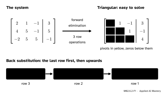
Elimination at a glance. Forward elimination turns the system into a triangular one with the same solutions. Back substitution then solves the triangular system from the bottom row up.

To save writing we drop the letters and keep the numbers. The augmented matrix of a system holds the coefficients, with the right-hand sides as one extra column after a bar. Each row is one equation: the row \({[\,2 \;\; 1 \;\; {-1} \mid 3\,]}\) stands for \(2x + y - z = 3\).

Build it up

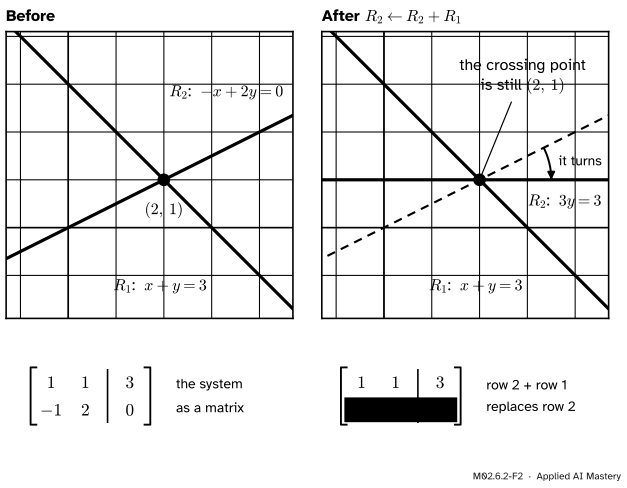
Step 1. The key move, in a picture. Take the system of the last lesson, \(x + y = 3\) and \(-x + 2y = 0\). Call its equations row 1 and row 2, or \(R_1\) and \(R_2\). Add row 1 to row 2 and put the result in place of row 2. We write this \({R_2 \leftarrow R_2 + R_1}\). The left-hand sides add to \({(-x + 2y)} + {(x + y)} = 3y\) and the right-hand sides add to \(0 + 3 = 3\). Row 2 is now \(3y = 3\).

M02.6.2-F2

One row operation, seen as lines and as a matrix. Adding row 1 to row 2 turns the second line about the crossing point until it is level. The unknown \(x\) has gone from row 2, and the solution has not moved.

The picture shows why the move is safe. At the crossing point both old equations are true, and adding two true equations gives a true equation. So the new line passes through the same point. What has changed is that row 2 no longer contains \(x\): we have eliminated it.

Step 2. The three moves. Elimination uses three row operations.

• Swap two rows, written \({R_i \leftrightarrow R_j}\). The equations are the same, in a new order.
• Scale a row by a number \(c\) that is not zero, written \({R_i \leftarrow cR_i}\). The equation \(2x + 2y = 6\) describes the same line as \(x + y = 3\).
• Replace a row by itself plus a multiple of another row, written \({R_i \leftarrow R_i + cR_j}\). This is the move in the figure.

Step 3. Use the moves in a fixed order. Work on one column at a time, from the left. In each column pick a pivot: a non-zero entry that will be used to clear the entries below it. For an entry \(a\) below a pivot \(p\), the multiplier is \(m = a/p\), and the operation \({R_i \leftarrow R_i - mR_k}\) (with the pivot in row \(k\)) turns that entry into \(a - (a/p)\,p = 0\). Clear the first column below its pivot, then the second column below its pivot, and so on. This is forward elimination, and it ends with a triangular system.

Step 4. Climb back up. Solve the last equation, put its answer into the one above, and continue to the top. This is back substitution.

The formal statement

NoteDefinition: augmented matrix and row operations

The augmented matrix of \(\mat{A}\vect{x} = \vect{b}\) is \({[\,\mat{A} \mid \vect{b}\,]}\): the matrix \(\mat{A}\) with \(\vect{b}\) attached as one more column. The three row operations are

\[ \begin{aligned} \text{swap:}\quad & R_i \leftrightarrow R_j \\ \text{scale:}\quad & R_i \leftarrow c\,R_i, \;\; c \neq 0 \\ \text{replace:}\quad & R_i \leftarrow R_i + c\,R_j, \;\; i \neq j \end{aligned} \]

NoteResult: row operations keep the solutions

Applying a row operation to an augmented matrix does not change the solution set of its system.

Proof. Write \(\ell_i(\vect{x})\) for the left-hand side of equation \(i\), so that equation \(i\) says \(\ell_i(\vect{x}) = b_i\). We show, for each operation, that \(\vect{x}\) solves the old system exactly when it solves the new one.

Swap. The new system has the same equations in a different order. A vector satisfies all of them in one order exactly when it satisfies all of them in the other.

Scale. Only equation \(i\) changes, to \(c\,\ell_i(\vect{x}) = c\,b_i\). If \(\ell_i(\vect{x}) = b_i\), multiplying both sides by \(c\) gives the new equation. If the new equation holds, dividing both sides by \(c\) gives the old one. The division is allowed because \(c \neq 0\).

Replace. Only equation \(i\) changes, to \(\ell_i(\vect{x}) + c\,\ell_j(\vect{x}) = b_i + c\,b_j\). Equation \(j\) is in both systems. Suppose \(\vect{x}\) solves the old system. Then \(\ell_i(\vect{x}) = b_i\) and \(\ell_j(\vect{x}) = b_j\), so

\[ \ell_i(\vect{x}) + c\,\ell_j(\vect{x}) = b_i + c\,b_j , \]

which is the new equation \(i\). Now suppose \(\vect{x}\) solves the new system. Then the displayed equation holds and so does \(\ell_j(\vect{x}) = b_j\). Subtract \(c\) times the second from the first:

\[ \ell_i(\vect{x}) = \big(b_i + c\,b_j\big) - c\,b_j = b_i , \]

which is the old equation \(i\). So the two systems have the same solutions. \(\blacksquare\)

Each half of the proof undoes the other. That is the real reason elimination works: every row operation can be reversed by another row operation of the same kind. A swap is undone by the same swap, scaling by \(c\) is undone by scaling by \(1/c\), and adding \(c\,R_j\) is undone by adding \(-c\,R_j\). Scaling by zero is banned because it cannot be undone: it wipes an equation out.

Forward elimination. For a system of \(n\) equations in \(n\) unknowns, repeat for \(k = 1, 2, \dots, n - 1\):

1. The pivot is the entry in row \(k\), column \(k\). If it is zero, swap row \(k\) with a lower row whose entry in column \(k\) is not zero.
2. For each row \(i\) below row \(k\), compute the multiplier \(m = a_{ik}/a_{kk}\) and apply \({R_i \leftarrow R_i - mR_k}\).

The result is an upper triangular system \(\mat{U}\vect{x} = \vect{c}\): every entry of \(\mat{U}\) below the diagonal is zero. If some column offers no non-zero entry to swap in, or the last diagonal entry \(u_{nn}\) is zero, the method stops, and the next lesson explains what that means.

Back substitution. Row \(i\) of the triangular system says

\[ \begin{aligned} &u_{ii}x_i + u_{i,i+1}x_{i+1} \\ &\quad {} + \cdots + u_{in}x_n = c_i . \end{aligned} \]

Work from \(i = n\) up to \(i = 1\). When row \(i\) is reached, the unknowns \(x_{i+1}, \dots, x_n\) are already known. Move their terms to the right and divide by the pivot \(u_{ii}\), which is not zero:

\[ x_i = \frac{c_i - u_{i,i+1}x_{i+1} - \cdots - u_{in}x_n}{u_{ii}}. \]

The whole method, forward elimination and then back substitution, is called Gaussian elimination.

Worked example

Solve this system.

\[ \begin{aligned} 2x + y - z &= 3 \\ 4x + 5y - z &= 5 \\ -2x + 5y + 5z &= -1 \end{aligned} \]

Its augmented matrix is

\[ \left[\begin{array}{rrr|r} 2 & 1 & -1 & 3 \\ 4 & 5 & -1 & 5 \\ -2 & 5 & 5 & -1 \end{array}\right] \]

M02.6.2-F3

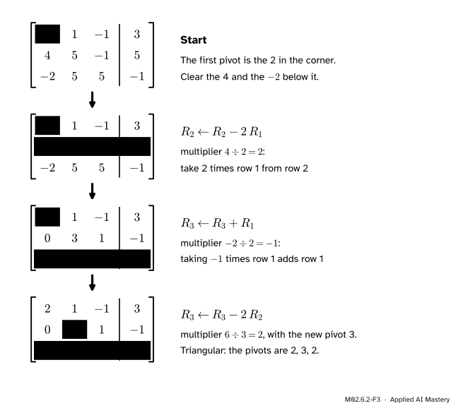
Forward elimination on the worked example. Yellow marks the pivot in use. Green marks the row that the operation has just rewritten.

Column 1. The pivot is the 2 in row 1.

Row 2 has a 4 under the pivot, so the multiplier is \(4/2 = 2\) and the operation is \({R_2 \leftarrow R_2 - 2R_1}\). It gives \({(0,\; 3,\; 1 \mid -1)}\), entry by entry, including the right-hand side:

\[ \begin{aligned} 4 - 2 \cdot 2 &= 0, \\ 5 - 2 \cdot 1 &= 3, \\ -1 - 2 \cdot (-1) &= 1, \\ 5 - 2 \cdot 3 &= -1. \end{aligned} \]

Row 3 has a \(-2\) under the pivot, so the multiplier is \(-2/2 = -1\). Subtracting \(-1\) times row 1 is the same as adding row 1, so the operation is \({R_3 \leftarrow R_3 + R_1}\), which gives \({(0,\; 6,\; 4 \mid 2)}\):

\[ \begin{aligned} -2 + 2 &= 0, \\ 5 + 1 &= 6, \\ 5 + (-1) &= 4, \\ -1 + 3 &= 2. \end{aligned} \]

Column 2. The pivot is the 3 now in row 2. Row 3 has a 6 under it, so the multiplier is \(6/3 = 2\) and the operation is \({R_3 \leftarrow R_3 - 2R_2}\), which gives \({(0,\; 0,\; 2 \mid 4)}\):

\[ \begin{aligned} 0 - 2 \cdot 0 &= 0, \\ 6 - 2 \cdot 3 &= 0, \\ 4 - 2 \cdot 1 &= 2, \\ 2 - 2 \cdot (-1) &= 4. \end{aligned} \]

The matrix is now triangular, with pivots 2, 3 and 2:

\[ \left[\begin{array}{rrr|r} 2 & 1 & -1 & 3 \\ 0 & 3 & 1 & -1 \\ 0 & 0 & 2 & 4 \end{array}\right] \]

Read as equations, its rows are \(2x + y - z = 3\), then \(3y + z = -1\), then \(2z = 4\). It is the easy system from the start of the lesson.

M02.6.2-F4

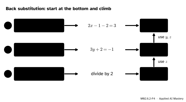
Back substitution on the triangular system. Each value found is carried up into the rows above it.

Back substitution.

Row 3: \(2z = 4\), so \(z = 2\).

Row 2: \(3y + z = -1\) becomes \(3y + 2 = -1\), so \(3y = -3\) and \(y = -1\).

Row 1: \(2x + y - z = 3\) becomes \(2x - 1 - 2 = 3\), so \(2x = 6\) and \(x = 3\).

Check in the original equations. \({2 \cdot 3} + (-1) - 2 = 3\). Then \({4 \cdot 3} + {5 \cdot (-1)} - 2 = 12 - 5 - 2 = 5\). Then \({-2 \cdot 3} + {5 \cdot (-1)} + {5 \cdot 2} = -6 - 5 + 10 = -1\). All three hold, so the solution is \((x, y, z) = (3, -1, 2)\). In the row picture, three planes meet at that one point.

Code

From scratch, with every row operation written out.

import numpy as np

def forward_eliminate(A, b):
    """Return the triangular system (U, c) with the same solutions, and a log of the operations."""
    M = np.column_stack([A, b]).astype(float)        # the augmented matrix [A | b]
    n = len(b)
    log = []
    for k in range(n):                               # column k, with its pivot in row k
        if M[k, k] == 0:                             # a zero where the pivot should be
            lower = [i for i in range(k + 1, n) if M[i, k] != 0]
            if not lower:
                raise ValueError(f"no pivot in column {k + 1}")
            M[[k, lower[0]]] = M[[lower[0], k]]      # swap in a row that has a non-zero entry
            log.append(f"R{k + 1} <-> R{lower[0] + 1}")
        for i in range(k + 1, n):
            if M[i, k] == 0:
                continue
            m = M[i, k] / M[k, k]                    # the multiplier
            M[i] = M[i] - m * M[k]                   # the whole row, right-hand side included
            log.append(f"R{i + 1} <- R{i + 1} - ({m:g}) R{k + 1}")
    return M[:, :n], M[:, n], log

def back_substitute(U, c):
    n = len(c)
    x = np.zeros(n)
    for i in range(n - 1, -1, -1):                   # the last row first
        known = sum(U[i, j] * x[j] for j in range(i + 1, n))
        x[i] = (c[i] - known) / U[i, i]
    return x

A = np.array([[2, 1, -1], [4, 5, -1], [-2, 5, 5]])
b = np.array([3, 5, -1])

U, c, log = forward_eliminate(A, b)
print("\n".join(log))
print(U)
print("c =", c)
x = back_substitute(U, c)
print("x =", x)

R2 <- R2 - (2) R1
R3 <- R3 - (-1) R1
R3 <- R3 - (2) R2
[[ 2.  1. -1.]
 [ 0.  3.  1.]
 [ 0.  0.  2.]]
c = [ 3. -1.  4.]
x = [ 3. -1.  2.]

The log repeats the worked example: multipliers 2, \(-1\) and 2, then \(\mat{U}\) and \(\vect{c}\) as in the last matrix of the trace, then \((3, -1, 2)\). The library call does all of it at once.

print(np.linalg.solve(A, b))

# A system that needs a row swap (exercise 2 below).
A2 = np.array([[1, 2, 1], [2, 4, 3], [1, 3, 2]])
b2 = np.array([4, 7, 5])
U2, c2, log2 = forward_eliminate(A2, b2)
print("\n".join(log2))
print("x =", back_substitute(U2, c2))

[ 3. -1.  2.]
R2 <- R2 - (2) R1
R3 <- R3 - (1) R1
R2 <-> R3
x = [ 1.  2. -1.]

One caution. The from-scratch code tests whether a pivot is exactly zero. That is fine for small whole numbers, but in floating-point arithmetic a pivot can be tiny without being zero, and dividing by it magnifies rounding errors. Library code guards against this by swapping the entry of largest absolute value in the column into the pivot position at every step, as lesson M02.6.4 explains.

Explore

M02.6-X1

Elimination stepper

Press Next step to apply one row operation at a time, and watch the matrix and the picture change together. The read-out names each operation and tells you what the planes or lines still have in common. You can also build your own row operation with the three sliders.

Things to try:

1. Press Two lines, then Next step once. Row 2 turns level, as in the figure above. Did the crossing point move?
2. Press Lesson system and step three times. These are the three operations of the worked example. Compare each matrix with the trace figure, and watch plane 3 end up level: \(2z = 4\).
3. Keep stepping. The stepper now carries out back substitution as row operations: it divides a row by its pivot and uses that row to clear the entries above the pivot. It stops when the matrix reads \(x = 3\), \(y = -1\), \(z = 2\). What do the three planes look like then?
4. Press Reset and use your own operation to do the second step of the worked example before the first: change row 3, use row 1, multiplier 1. Then let Next step finish. Does the answer change?
5. Press Needs a swap and step. What does the stepper do at the third step, and why?

Carrying the row operations on until every pivot is 1 and stands alone in its column, as the stepper does, is called Gauss-Jordan elimination. By hand, back substitution is less work.

Pitfalls

M02.6.2-F5

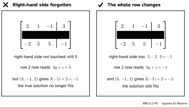
Wrong beside right. A row operation acts on a whole equation. Leave the right-hand side behind and the new row describes a different plane, one that misses the true solution.

“Row operations are done to the matrix of coefficients. The right-hand side stays as it is.”

A row is an equation, and an equation has two sides. In the figure, forgetting to update the 5 turns the true equation \(3y + z = -1\) into \(3y + z = 5\), which the solution \((3, -1, 2)\) does not satisfy. Writing the augmented matrix, bar and all, is the habit that prevents this.

“A zero in the pivot position means the system cannot be solved.”

Not yet. Look down the column first. If a lower row has a non-zero entry there, swap the rows and carry on, as in exercise 2. Only when the whole column below is zero does something new happen, and that is the subject of the next lesson.

“I can save time by doing two replacements at once.”

Each operation must use the rows as they are now. Suppose you apply \({R_2 \leftarrow R_2 - R_3}\) and \({R_3 \leftarrow R_3 - R_2}\) together, both from the old rows. The new rows are negatives of each other, so one equation has been lost and the new system can have solutions that the old one did not. Done one after the other, the two operations are safe.

“Elimination is a classroom method. Real software does something cleverer.”

For a general square system, real software does exactly this. A call to numpy.linalg.solve runs forward elimination with row swaps and then back substitution, organised as lesson M02.6.4 describes.

Check yourself

Recall

1. What does one row of an augmented matrix stand for?

Show answer

One equation of the system. The entries before the bar are the coefficients of the unknowns and the entry after the bar is the right-hand side.

2. Name the three row operations.

Show answer

Swap two rows. Scale a row by a non-zero number. Replace a row by itself plus a multiple of another row.

3. Why does a row operation never change the solution set?

Show answer

Any vector that solves the old system solves the new one, and each operation can be undone by an operation of the same kind, so any vector that solves the new system solves the old one too.

4. A pivot is 3 and the entry below it is 6. What is the multiplier, and which operation clears the 6?

Show answer

The multiplier is \(6/3 = 2\). Subtract 2 times the pivot row from the lower row: the entry becomes \(6 - {2 \cdot 3} = 0\).

5. In back substitution, which equation is solved first, and why?

Show answer

The last one. In a triangular system it contains a single unknown. Each row above it then has only one unknown that is not yet known.

Exercises

1. ★ Solve \(3x + 2y = 7\), \(6x + 5y = 16\) by elimination. Name the pivot and the multiplier.

Show solution

The augmented matrix is \(\left[\begin{array}{rr|r} 3 & 2 & 7 \\ 6 & 5 & 16 \end{array}\right]\). The pivot is 3 and the multiplier is \(6/3 = 2\). The operation \({R_2 \leftarrow R_2 - 2R_1}\) gives the row \({(6 - 6,\; 5 - 4 \mid 16 - 14)} = {(0,\; 1 \mid 2)}\).

Back substitution: \(y = 2\). Then \(3x + {2 \cdot 2} = 7\), so \(3x = 3\) and \(x = 1\).

Check: \(3 + 4 = 7\) and \(6 + 10 = 16\).

2. ★★ Solve the system below by elimination. You will need a row swap.

\[ \begin{aligned} x + 2y + z &= 4 \\ 2x + 4y + 3z &= 7 \\ x + 3y + 2z &= 5 \end{aligned} \]

Show solution

Start from \(\left[\begin{array}{rrr|r} 1 & 2 & 1 & 4 \\ 2 & 4 & 3 & 7 \\ 1 & 3 & 2 & 5 \end{array}\right]\).

Column 1, pivot 1. \({R_2 \leftarrow R_2 - 2R_1}\) gives \({(0,\; 0,\; 1 \mid -1)}\). \({R_3 \leftarrow R_3 - R_1}\) gives \({(0,\; 1,\; 1 \mid 1)}\).

Column 2. The pivot position, row 2 column 2, holds a zero. Row 3 has a 1 in that column, so swap: \({R_2 \leftrightarrow R_3}\). The matrix is now

\[ \left[\begin{array}{rrr|r} 1 & 2 & 1 & 4 \\ 0 & 1 & 1 & 1 \\ 0 & 0 & 1 & -1 \end{array}\right], \]

which is already triangular.

Back substitution: \(z = -1\). Then \(y + (-1) = 1\), so \(y = 2\). Then \(x + {2 \cdot 2} + (-1) = 4\), so \(x = 1\). The solution is \((1, 2, -1)\).

Check: \(1 + 4 - 1 = 4\), then \(2 + 8 - 3 = 7\), then \(1 + 6 - 2 = 5\).

3. ★★★ Show that a swap is not really a separate operation: the rows \(R_1\) and \(R_2\) can be exchanged using only the other two kinds of row operation.

Show solution

Let the two rows start as \(\vect{p}\) and \(\vect{q}\). Apply four operations in turn.

1. \({R_1 \leftarrow R_1 + R_2}\). The rows are \(\vect{p} + \vect{q}\) and \(\vect{q}\).
2. \({R_2 \leftarrow R_2 - R_1}\). The rows are \(\vect{p} + \vect{q}\) and \(\vect{q} - {(\vect{p} + \vect{q})} = -\vect{p}\).
3. \({R_1 \leftarrow R_1 + R_2}\). The rows are \({(\vect{p} + \vect{q})} - \vect{p} = \vect{q}\) and \(-\vect{p}\).
4. \({R_2 \leftarrow (-1)R_2}\). The rows are \(\vect{q}\) and \(\vect{p}\).

Three replacements and one scaling by \(-1\) did the work of one swap. The swap is kept as an operation of its own because it is so much shorter.

Summary card

Make it triangular without changing the solutions, then climb back up.

M02.6.2-F1

Eliminate forwards, substitute backwards.

• Row operations. Swap, scale by \({c \neq 0}\), replace by \({R_i + cR_j}\). None changes the solution set.
• Multiplier. To clear an entry \(a\) under a pivot \(p\), subtract \({m = a/p}\) times the pivot row.
• Zero pivot. Swap in a lower row with a non-zero entry in that column.
• Back substitution. For \(i = n\) down to 1, \(x_i\) is \(c_i\) minus the terms already known, divided by the pivot \(u_{ii}\).

Sources and next steps

Sources. Each was opened and checked against this lesson on 12 November 2026.

• Gilbert Strang, Elimination with matrices, MIT OpenCourseWare 18.06SC, with its lecture summary. The section “Method of Elimination” defines pivots and multipliers on a three-by-three example, augments the matrix with \(\vect{b}\), reaches \(\mat{U}\vect{x} = \vect{c}\) and solves it by back substitution. It also gives the rule for a zero in the pivot position: exchange with a row below. The section “Elimination Matrices” gives the reason the method works: all steps can be reversed.
• Dan Margalit and Joseph Rabinoff, Interactive Linear Algebra, Section 1.2, Row Reduction, Georgia Institute of Technology (open access). It lists the three row operations under the names scaling, replacement and swap, defines a pivot, and states that row operations do not change the solution set.

Next. M02.6.3 None, one, or infinitely many asks what elimination shows when a column has no pivot to offer.

This lesson unlocks

M02.6.3 None, one, or infinitely many

Your progress is saved in this browser only. No account, no tracking.