Apply one linear map to the result of another and you get a third linear map. Prove it, find the matrix of the combined map by following the two basis vectors through both steps, and learn why a product of matrices is read from right to left.
Define the composition of two maps and say which map acts first, both in the notation for maps and in a product of two matrices.
Prove that the composition of two linear maps is a linear map.
Find the matrix of a composition by following the two basis vectors through both maps.
Check a composition on a vector in two ways: by applying the two maps in turn, and by applying the single combined matrix.
In review. The maths and code on this page are checked by automated tests on every change, but an independent reader has not signed it off yet. Spot a mistake or a confusing step? Tell us.
The question
A photo editor slants a picture and then turns it. A neural network multiplies its input by one matrix, then by another, then by another. Each step on its own is a linear map. Is the whole chain still a linear map? And if it is, which single matrix does in one go what the chain does in several?
Intuition
To compose two maps is to do one and then feed its output to the other. That is all.
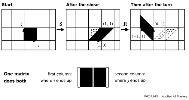
Take two maps from M02.4.3. The shear holds the horizontal axis still and slides everything above it sideways. The quarter turn rotates the plane by \(90°\) anticlockwise. Do the shear first, then the turn.
M02.5.1-F1
A shear \(\mat{S}\), then a quarter turn \(\mat{R}\). Each panel shows where the unit square, the letter F and the two basis vectors are at that moment. The matrix underneath does both steps at once: its columns are the two arrows of the last panel.
Look at the last panel and ask the questions of M02.4.1. Are the grid lines still straight, parallel and evenly spaced? Yes: the shear turns a grid into a grid, and the turn does the same to whatever grid it is handed. Is the origin where it was? Yes: neither step moved it.
So the two steps together behave like one linear map. If that is right, the combined map has a matrix, and M02.4.2 says what its columns must be: the places where \(\ihat\) and \(\jhat\) end up. Read them off the last panel: \((0, 1)\) and \((-1, 1)\).
This lesson makes that argument watertight, and turns “read them off the picture” into a calculation.
Build it up
Step 1. Name the two maps. From M02.4.3, the shear and the quarter turn have the matrices
The columns of \(\mat{S}\) say that the shear leaves \(\ihat\) at \((1, 0)\) and sends \(\jhat\) to \((1, 1)\). The columns of \(\mat{R}\) say that the turn sends \(\ihat\) to \((0, 1)\) and \(\jhat\) to \((-1, 0)\).
Step 2. Do one, then the other, to a single vector. Take \(\vect{v} = (2, 1)\). The shear gives
The second map never sees \(\vect{v}\). It sees only what the first map made of it.
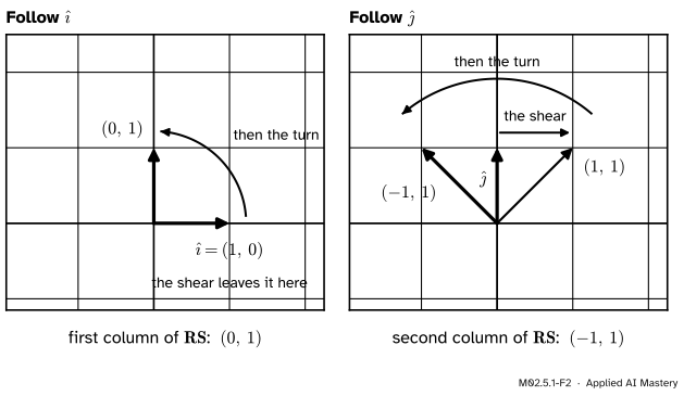
Step 3. Follow \(\ihat\) through both maps. The shear leaves \(\ihat\) at \((1, 0)\), the first column of \(\mat{S}\). The turn then sends \((1, 0)\) to \((0, 1)\), the first column of \(\mat{R}\).
Step 4. Follow \(\jhat\) through both maps. The shear sends \(\jhat\) to \((1, 1)\), the second column of \(\mat{S}\). The turn then acts on \((1, 1)\):
Test it on \(\vect{v} = (2, 1)\) with one multiplication: \(2\,(0, 1) + 1\,(-1, 1) = (-1, 3)\). That is the answer of Step 2, reached in one step where Step 2 took two.
Step 6. Give the new matrix a name. It is called the product of \(\mat{R}\) and \(\mat{S}\) and is written \(\mat{R}\mat{S}\). Notice the order. The map that acts first is written on the right, because in \(\mat{R}(\mat{S}\vect{v})\) the matrix \(\mat{S}\) stands next to the vector.
The formal statement
NoteDefinition: composition
Let \(T_1 : \R^p \to \R^n\) and \(T_2 : \R^n \to \R^m\) be maps. Their composition is the map \(T_2 \circ T_1 : \R^p \to \R^m\) given by
Read \(T_2 \circ T_1\) as “\(T_2\) after \(T_1\)”. The map \(T_1\) acts first.
The composition makes sense only when every output of \(T_1\) is a valid input of \(T_2\). Here both are vectors with \(n\) entries. In the plane \(p = n = m = 2\) and nothing can go wrong. Lesson M02.5.4 looks at the other cases.
NoteResult 1: a composition of linear maps is linear
If \(T_1\) and \(T_2\) are linear maps, then \(T_2 \circ T_1\) is a linear map.
Proof. By Consequence 2 of M02.4.1 it is enough to check the combined rule. Take vectors \(\vect{u}, \vect{v}\) and numbers \(a, b\).
The first and last steps are the definition of composition. The second step holds because \(T_1\) is linear. In the third, \(T_2\) is applied to a combination of the two vectors \(T_1(\vect{u})\) and \(T_1(\vect{v})\), and its own linearity lets the numbers \(a\) and \(b\) pass through. So the combined rule holds, and the composition is linear.
NoteResult 2: the matrix of a composition
Let \(T_1\) be the map of the matrix \(\mat{B}\), with columns \(\vect{b}_1\) and \(\vect{b}_2\), and let \(T_2\) be the map of the matrix \(\mat{A}\). Then the matrix of \(T_2 \circ T_1\) has the columns \(\mat{A}\vect{b}_1\) and \(\mat{A}\vect{b}_2\).
Proof. By Result 1 the composition is linear, so by M02.4.2 it has exactly one matrix, and the columns of that matrix are the images of \(\ihat\) and \(\jhat\). For \(\ihat\):
The first step is the definition of composition. The second uses \(T_1(\ihat) = \mat{B}\,\ihat =
\vect{b}_1\): multiplying a matrix by \(\ihat\) picks out its first column (M02.4.2). The third says that \(T_2\) is multiplication by \(\mat{A}\). In the same way \(\jhat\) ends up at \(\mat{A}\vect{b}_2\).
NoteDefinition: the product of two matrices
The product\(\mat{A}\mat{B}\) is the matrix of “first \(\mat{B}\), then \(\mat{A}\)”. Its columns are \(\mat{A}\) applied to the columns of \(\mat{B}\):
The last equation is not an extra assumption. \(\mat{A}\mat{B}\) was built to be the matrix of the map \(\vect{v} \mapsto \mat{A}(\mat{B}\vect{v})\), and “the matrix of a map” means exactly that multiplying by it gives the map’s output.
Read a product from right to left. In \(\mat{A}\mat{B}\vect{v}\) the matrix nearest the vector acts first. The habit comes from the way functions are written: in \(f(g(x))\) the inner function \(g\) is on the right, and it is applied first.
In any number of dimensions the argument is the same, with the basis vectors \(\vect{e}_1, \dots, \vect{e}_p\) in place of \(\ihat\) and \(\jhat\): column \(j\) of \(\mat{A}\mat{B}\) is \(\mat{A}\vect{b}_j\). The next lesson turns this into a rule for every entry.
Go deeper: a later map cannot bring back what an earlier one destroyed
Suppose the first map sends some non-zero vector \(\vect{d}\) to zero: \(T_1(\vect{d}) = \vect{0}\). Then, whatever the second map is,
because every linear map sends \(\vect{0}\) to \(\vect{0}\) (Consequence 1 of M02.4.1). The composition loses \(\vect{d}\) too.
For example, project onto the horizontal axis with \(\mat{P} = \begin{bmatrix} 1 & 0 \\ 0 & 0 \end{bmatrix}\), then make a quarter turn. Follow the basis vectors: \(\ihat \to (1, 0) \to (0, 1)\) and \(\jhat \to (0, 0) \to (0, 0)\). So
which sends \((x, y)\) to \((0, x)\). The whole plane lands on the vertical axis. The turn moved the flattened plane but could not unflatten it. In a neural network the same thing holds: what one layer throws away, no later layer can recover. M02.7 makes this precise with the idea of rank.
Worked example
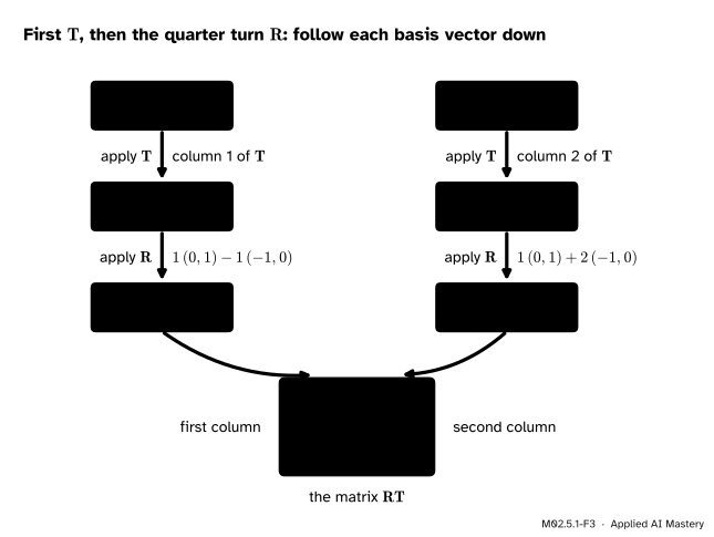
The map of M02.4 is \(T(x, y) = (x + y,\; -x + 2y)\), with matrix \(\mat{T} = \begin{bmatrix} 1 & 1 \\ -1 & 2 \end{bmatrix}\). Apply \(\mat{T}\) first and the quarter turn \(\mat{R}\) second. Find the matrix of the composition, \(\mat{R}\mat{T}\).
M02.5.1-F3
The worked example as a trace. Each basis vector goes down through \(\mat{T}\) and then through \(\mat{R}\). The two results are the columns of \(\mat{R}\mat{T}\).
Follow \(\ihat\). First \(\mat{T}\): the image of \(\ihat\) is the first column of \(\mat{T}\), which is \((1, -1)\). Then \(\mat{R}\):
Check on a vector. Take \(\vect{v} = (2, 1)\). In two steps: \(\mat{T}\vect{v} = (3, 0)\), as in M02.4.1, and then \(\mat{R}\,(3, 0) = 3\,(0, 1) + 0\,(-1, 0) = (0, 3)\). In one step:
The other order, as a warning. Turn first and apply \(\mat{T}\) second. Then \(\ihat\) goes to \((0, 1)\) and on to \(\mat{T}\,(0, 1) = (1, 2)\), and \(\jhat\) goes to \((-1, 0)\) and on to \(\mat{T}\,(-1, 0) = -1\,(1, -1) = (-1, 1)\):
The order of the two maps matters. Lesson M02.5.3 is about that.
Code
First from scratch. A map is a Python function, and composing two maps is one line.
def matvec(A, v):"""Matrix times vector: v[0] of the first column plus v[1] of the second (M02.4.2)."""return [v[0] * A[0][0] + v[1] * A[0][1], v[0] * A[1][0] + v[1] * A[1][1]]def compose(second, first):"""The map 'first, then second'. The arguments are in the order of second(first(v))."""returnlambda v: second(first(v))def matrix_of(f):"""The matrix of a linear map of the plane: its columns are f(i-hat) and f(j-hat).""" c1, c2 = f([1, 0]), f([0, 1])return [[c1[0], c2[0]], [c1[1], c2[1]]]S = [[1, 1], [0, 1]] # the shearR = [[0, -1], [1, 0]] # the quarter turnshear =lambda v: matvec(S, v)turn =lambda v: matvec(R, v)shear_then_turn = compose(turn, shear)RS = matrix_of(shear_then_turn)print("two steps on (2, 1):", shear([2, 1]), "->", shear_then_turn([2, 1]))print("matrix of the composition:", RS)print("one step on (2, 1): ", matvec(RS, [2, 1]))
two steps on (2, 1): [3, 1] -> [-1, 3]
matrix of the composition: [[0, -1], [1, 1]]
one step on (2, 1):  [-1, 3]
The worked example, and the same two maps in the other order:
T = [[1, 1], [-1, 2]]apply_T =lambda v: matvec(T, v)RT = matrix_of(compose(turn, apply_T)) # first T, then the turnTR = matrix_of(compose(apply_T, turn)) # first the turn, then Tprint("first T, then the turn:", RT, " on (2, 1):", matvec(RT, [2, 1]))print("first the turn, then T:", TR)
first T, then the turn: [[1, -2], [1, 1]]   on (2, 1): [0, 3]
first the turn, then T: [[1, -1], [2, 1]]
Now NumPy, where the product of two matrices is written A @ B. The loop tests both results of this lesson on a thousand random pairs of matrices.
import numpy as npS, R = np.array([[1, 1], [0, 1]]), np.array([[0, -1], [1, 0]])v = np.array([2, 1])print("R @ (S @ v) =", R @ (S @ v), " two steps")print("(R @ S) @ v =", (R @ S) @ v, " one step with the product")print("R @ S =", (R @ S).tolist())rng = np.random.default_rng(0)for _ inrange(1000): A, B = rng.normal(size=(2, 2)), rng.normal(size=(2, 2)) u, w = rng.normal(size=2), rng.normal(size=2) a, b = rng.normal(size=2) both =lambda x: A @ (B @ x) # first B, then Aassert np.allclose(both(a * u + b * w), a * both(u) + b * both(w)) # Result 1: it is linearassert np.allclose((A @ B)[:, 0], A @ B[:, 0]) # Result 2: column 1assert np.allclose((A @ B)[:, 1], A @ B[:, 1]) # Result 2: column 2assert np.allclose((A @ B) @ u, both(u)) # the product does both stepsprint("1000 random pairs: the composition is linear, and A @ B is its matrix")
R @ (S @ v) = [-1  3]   two steps
(R @ S) @ v = [-1  3]   one step with the product
R @ S = [[0, -1], [1, 1]]
1000 random pairs: the composition is linear, and A @ B is its matrix
Explore
This module’s interactive, the composition explorer, lives in lesson M02.5.3. If you would like to see this lesson’s picture move now, open it and press Step twice: once for the shear, once for the turn. The read-out shows where \(\ihat\) and \(\jhat\) are after each step, and the single matrix that does both.
Pitfalls
M02.5.1-F4
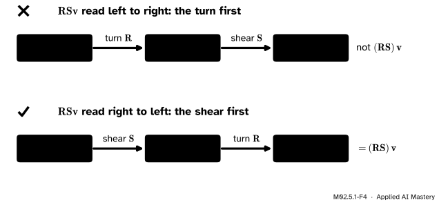
Wrong beside right. In \(\mat{R}\mat{S}\vect{v}\) the shear stands next to the vector, so the shear acts first. Reading the product from left to right applies the maps in the wrong order and lands somewhere else.
“\(\mat{R}\mat{S}\) means: do \(\mat{R}\), then \(\mat{S}\).”
We read text from left to right, so this is the natural guess, and it is wrong. The product \(\mat{R}\mat{S}\) is defined by \((\mat{R}\mat{S})\vect{v} = \mat{R}(\mat{S}\vect{v})\): the matrix next to the vector acts first. Code often runs the other way. In PyTorch, nn.Sequential(layer1, layer2) lists the layers in the order in which they run, so the layer written first acts first. As matrices, the same network is \(\mat{W}_2\mat{W}_1\), with the first layer on the right.
“To do two maps one after the other, add their matrices.”
Adding matching entries gives \(\mat{R} + \mat{S} = \begin{bmatrix} 1 & 0 \\ 1 & 1 \end{bmatrix}\), and this matrix sends \(\vect{v}\) to \(\mat{R}\vect{v} + \mat{S}\vect{v}\). That applies each map to the original vector and adds the two results. Nothing is fed into anything. For \(\vect{v} = (2, 1)\) it gives \((2, 3)\), where the shear followed by the turn gives \((-1, 3)\).
“The second map follows the grid that the first map moved.”
After the quarter turn it is tempting to picture the shear sliding things along the turned grid lines. It does not. Each matrix describes a map of the fixed plane: the shear always slides a point sideways, across the page, by an amount equal to its height above the horizontal axis. After the turn, \(\ihat\) sits at \((0, 1)\), at height 1, so the shear moves it to \((1, 1)\). Describing a map relative to a moved grid is a different idea, change of basis, and it has its own module, M02.9.
Check yourself
Recall
1. What does \(T_2 \circ T_1\) mean, and which map acts first?
Show answer
It is the map \(\vect{v} \mapsto T_2(T_1(\vect{v}))\), read “\(T_2\) after \(T_1\)”. \(T_1\) acts first.
2. Is the composition of two linear maps always linear? Which property of each map does the proof use?
Show answer
Yes. The proof uses the linearity of \(T_1\) and then the linearity of \(T_2\), each in the form of the combined rule \(T(a\vect{u} + b\vect{v}) = aT(\vect{u}) + bT(\vect{v})\).
3. How do you find the matrix of “first \(\mat{B}\), then \(\mat{A}\)”?
Show answer
Follow \(\ihat\) and \(\jhat\) through both maps and write where they end up as columns. The columns are \(\mat{A}\vect{b}_1\) and \(\mat{A}\vect{b}_2\): \(\mat{A}\) applied to the columns of \(\mat{B}\).
4. In the product \(\mat{A}\mat{B}\), which matrix acts first on a vector?
Show answer
\(\mat{B}\), the one on the right. \((\mat{A}\mat{B})\vect{v} = \mat{A}(\mat{B}\vect{v})\).
5. For the shear \(\mat{S}\) and the quarter turn \(\mat{R}\) of this lesson, what is \(\mat{R}\mat{S}\)?
Show answer
\(\begin{bmatrix} 0 & -1 \\ 1 & 1 \end{bmatrix}\). Its columns are where \(\ihat\) and \(\jhat\) end up after the shear and then the turn: \((0, 1)\) and \((-1, 1)\).
Exercises
1.★ Use the same two maps in the other order: first the quarter turn \(\mat{R}\), then the shear \(\mat{S}\). Follow \(\ihat\) and \(\jhat\) to find the matrix \(\mat{S}\mat{R}\). Is it the same as \(\mat{R}\mat{S}\)?
Show solution
\(\ihat\): the turn sends it to \((0, 1)\). The shear then gives \(\mat{S}\,(0, 1) = 0\,(1, 0) + 1\,(1, 1) = (1, 1)\).
\(\jhat\): the turn sends it to \((-1, 0)\). The shear then gives \(\mat{S}\,(-1, 0) = -1\,(1, 0) + 0\,(1, 1) = (-1, 0)\).
So \(\mat{S}\mat{R} = \begin{bmatrix} 1 & -1 \\ 1 & 0 \end{bmatrix}\). It is not \(\mat{R}\mat{S} = \begin{bmatrix} 0 & -1 \\ 1 & 1 \end{bmatrix}\). You have just found the subject of lesson M02.5.3.
2.★★ (a) Find the matrix of two quarter turns in a row, \(\mat{R}\mat{R}\), and say what map it is. (b) Let \(\mat{P} = \begin{bmatrix} 1 & 0 \\ 0 & 0 \end{bmatrix}\) be the projection onto the horizontal axis. Find the matrix of “first the quarter turn, then the projection”, and describe where it sends a point \((x, y)\).
Show solution
(a) \(\ihat \to (0, 1) \to \mat{R}\,(0, 1) = (-1, 0)\), and \(\jhat \to (-1, 0) \to \mat{R}\,(-1, 0) = -1\,(0, 1) = (0, -1)\). So \(\mat{R}\mat{R} = \begin{bmatrix} -1 & 0 \\ 0 & -1 \end{bmatrix}\): a half turn, which sends every vector to its opposite.
(b) \(\ihat \to (0, 1) \to \mat{P}\,(0, 1) = (0, 0)\), and \(\jhat \to (-1, 0) \to \mat{P}\,(-1, 0) = (-1, 0)\). So \(\mat{P}\mat{R} = \begin{bmatrix} 0 & -1 \\ 0 & 0 \end{bmatrix}\). It sends \((x, y)\) to \(x\,(0, 0) + y\,(-1, 0) = (-y, 0)\): the point is turned and then dropped onto the horizontal axis.
3.★★★ A neural-network layer is an affine map: a matrix followed by a shift. Let \(f(\vect{v}) = \mat{B}\vect{v} + \vect{p}\) and \(g(\vect{v}) = \mat{A}\vect{v} + \vect{q}\). Show that the composition \(g \circ f\) is again of the form “matrix times \(\vect{v}\), plus a fixed vector”, and find that matrix and that vector.
Show solution
Start from the definition of composition and substitute:
The last step uses \(\mat{A}(\mat{B}\vect{v}) = (\mat{A}\mat{B})\vect{v}\). So \(g \circ f\) is an affine map with matrix \(\mat{A}\mat{B}\) and shift \(\mat{A}\vect{p} + \vect{q}\). Two layers with nothing between them are one layer. Lesson M02.5.4 returns to this.
Summary card
One linear map after another is a linear map, and its matrix is where the basis vectors end up.
It stays linear. If \(T_1\) and \(T_2\) are linear, so is \(T_2 \circ T_1\).
Its matrix. The product \(\mat{A}\mat{B}\) has columns \(\mat{A}\vect{b}_1\) and \(\mat{A}\vect{b}_2\).
What it does.\((\mat{A}\mat{B})\vect{v} = \mat{A}(\mat{B}\vect{v})\) for every \(\vect{v}\).
Reading order. Right to left: the matrix next to the vector acts first.
Sources and next steps
Sources. Each was opened and checked against this lesson on 12 November 2026.
Sheldon Axler, Linear Algebra Done Right, 4th edition (open access). Section 3A, definition 3.7, defines the product of two linear maps by \((ST)(u) = S(Tu)\), notes that it is the usual composition \(S \circ T\), and asks the reader to verify that it is a linear map, which is Result 1 here. Section 3C, result 3.43, states that the matrix of a product of linear maps is the product of their matrices.
Grant Sanderson, Matrix multiplication as composition, 3Blue1Brown, Linear Algebra, chapter 4. The source of the method: follow \(\ihat\) and \(\jhat\) through both transformations to get the columns of the product, and read the product from right to left because that is how function notation works.
PyTorch documentation, torch.nn.Sequential. Modules are added in the order in which they are passed to the constructor, and the input goes to the first module, whose output is chained to the next.