A linear system Ax = b hands you the output of a linear map and asks for the input. See the same two equations as lines that cross and as columns that add up, and learn how to tell whether a target can be reached at all.
Rewrite a set of linear equations as one matrix equation, and name the coefficient matrix, the unknown vector and the target.
Read a linear system as a question about a map: which input lands on the target?
Draw the row picture of a two-by-two system and find the solution where the lines cross.
Draw the column picture of the same system and check a solution as a combination of the columns.
Decide whether a target can be reached by asking whether it lies in the span of the columns.
In review. The maths and code on this page are checked by automated tests on every change, but an independent reader has not signed it off yet. Spot a mistake or a confusing step? Tell us.
The question
A matrix is a machine: put a vector in and a vector comes out. Fitting a line to data, pricing a basket of goods and training a linear model all need the machine run backwards. You are handed the output and must find the input. How do you do that, and can it always be done?
Intuition
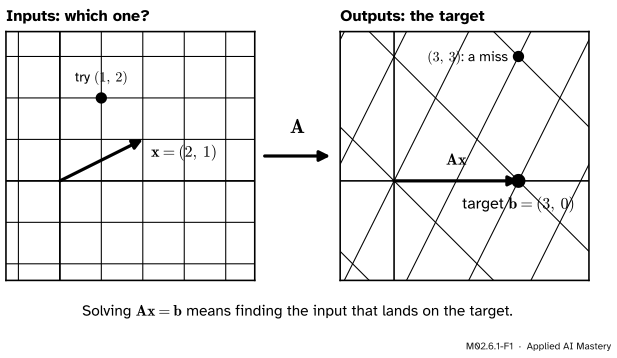
In module M02.4 a matrix \(\mat{A}\) was a map. It takes an input \(\vect{x}\) and gives the output \(\mat{A}\vect{x}\). A linear system asks the question the other way round. It names an output, which we call the target\(\vect{b}\), and asks which input lands there.
Take the course’s running map \(T(x, y) = {(x + y,\; -x + 2y)}\). Its matrix has the columns \((1, -1)\) and \((1, 2)\), the places where the two basis vectors land. Lesson M02.4.1 computed \(T(2, 1) = (3, 0)\). Now hide the input and keep only the output. “Which \(\vect{x}\) does the map send to \((3, 0)\)?” is a linear system.
M02.6.1-F1
A linear system gives you the output and asks for the input. The candidate \((1, 2)\) lands on \((3, 3)\) and misses. The input \((2, 1)\) lands exactly on the target \(\vect{b} = (3, 0)\), so it is the solution.
Guessing inputs one at a time is hopeless, because there are infinitely many to try. The rest of this module is about going straight to the answer. The first step is to look at the question in two more ways. Each shows something that the other hides.
Build it up
Step 1. Write the question as equations. The matrix of \(T\) is \(\mat{A} = \begin{bmatrix} 1 & 1 \\ -1 & 2 \end{bmatrix}\), and the unknown input is \(\vect{x} = (x, y)\). The question is
Multiply out the left-hand side one row at a time, as in lesson M02.4.2, and it becomes two ordinary equations that must both hold:
\[
\begin{aligned}
x + y &= 3 \\
-x + 2y &= 0 .
\end{aligned}
\]
So “several linear equations at once” and “one matrix equation” are the same thing.
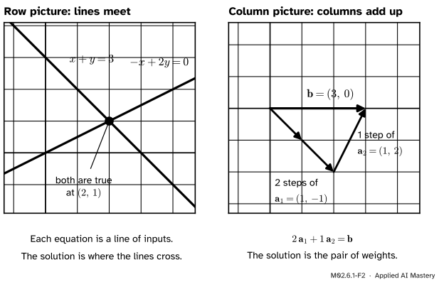
Step 2. The row picture. Look at one equation at a time. The first, \(x + y = 3\), is true for \((3, 0)\), for \((2, 1)\), for \((0, 3)\) and for every other point of one straight line. The second, \(-x + 2y = 0\), is true for the points of another line. A solution has to make both equations true, so it has to lie on both lines. They cross at one point, \((2, 1)\).
Step 3. The column picture. Now read the same product by columns. Lesson M02.4.2 showed that a matrix times a vector is a combination of the columns, weighted by the entries of the vector:
This asks a different-sounding question: how much of each column must be added together to reach the target? The answer is 2 of the first and 1 of the second.
M02.6.1-F2
The same system, drawn twice. Left: each equation is a line, and the solution is the point on both. Right: the columns of the matrix are arrows, and the solution is the pair of weights that carries them to \(\vect{b}\).
Both pictures give \(x = 2\) and \(y = 1\). They must, because they are two readings of the same two equations. But they are drawn in different places. The row picture lives in the input plane: its points are candidate inputs. The column picture lives in the output plane: its arrows are outputs of the map.
The formal statement
NoteDefinition: linear system
A linear system of \(m\) equations in \(n\) unknowns \(x_1, \dots, x_n\) is
\(\mat{A}\) is the \(m \times n\)coefficient matrix, \(\vect{x}\) in \(\R^n\) is the unknown vector and \(\vect{b}\) in \(\R^m\) is the right-hand side, which this module also calls the target. A solution is a vector \(\vect{x}\) that makes every equation true. The solution set is the collection of all solutions.
The one equation \(\mat{A}\vect{x} = \vect{b}\) can be read in three ways.
Reading 1: a question about a map. Let \(T(\vect{x}) = \mat{A}\vect{x}\). The solution set is the set of all inputs that \(T\) sends to \(\vect{b}\).
Reading 2: the row picture. Row \(i\) of the product is \(a_{i1}x_1 + \cdots + a_{in}x_n\), so row \(i\) of the system is one equation, \(a_{i1}x_1 + \cdots
+ a_{in}x_n = b_i\). With two unknowns its solutions form a line, as long as the two coefficients are not both zero. To see why, suppose \(a_{i2} \neq 0\) and solve for the second unknown: \(y = {(b_i - a_{i1}x)}/a_{i2}\), a straight-line graph. If \(a_{i2} = 0\) and \(a_{i1} \neq 0\), the equation says \(x = b_i/a_{i1}\), a vertical line. (An equation whose coefficients are all zero is not a line. Lesson M02.6.3 meets it.) With three unknowns each equation gives a plane, on the same condition. The solution set is what all the lines, or all the planes, have in common.
Reading 3: the column picture. Write \(\vect{a}_1, \dots, \vect{a}_n\) for the columns of \(\mat{A}\). Then \(\mat{A}\vect{x} = x_1\vect{a}_1 + \cdots + x_n\vect{a}_n\), so the system says
Two vectors are equal exactly when their coordinates are equal. So this vector equals \((b_1, b_2)\) exactly when \(a_{11}x + a_{12}y = b_1\) and \(a_{21}x + a_{22}y = b_2\), which are the two row equations. The same sum, coordinate by coordinate, works for any number of rows and columns.
When is there a solution at all? The column picture answers this in one line.
NoteResult: reachable targets
\(\mat{A}\vect{x} = \vect{b}\) has at least one solution exactly when \(\vect{b}\) is in the span of the columns of \(\mat{A}\).
Why. The span of the columns is the set of all their linear combinations (lesson M02.2.2). If \(\vect{x}\) is a solution, then \(\vect{b} = x_1\vect{a}_1 + \cdots + x_n\vect{a}_n\), which is a combination of the columns, so \(\vect{b}\) is in their span. In the other direction, if \(\vect{b}\) is in the span, then \(\vect{b} = c_1\vect{a}_1 + \cdots + c_n\vect{a}_n\) for some numbers \(c_1, \dots, c_n\), and the vector \(\vect{x} = (c_1, \dots, c_n)\) satisfies \(\mat{A}\vect{x} = \vect{b}\).
For the running map this settles everything. Its columns \((1, -1)\) and \((1, 2)\) are not multiples of each other, so their span is the whole plane and every target can be reached. They also form a basis of the plane, and coordinates in a basis are unique (lesson M02.2.4). So for every\(\vect{b}\) the system has exactly one solution.
Go deeper: a formula that runs this map backwards
Because every target has exactly one input, we can solve for a general target \((b_1, b_2)\) once and for all. The system is \(x + y = b_1\) and \(-x + 2y = b_2\). Add the two equations: the \(x\) terms cancel and \(3y = b_1 + b_2\), so \(y = \tfrac13{(b_1 + b_2)}\). Put that into the first equation: \(x = b_1 - y = b_1 - {\tfrac13(b_1 + b_2)} = {\tfrac13(2b_1 - b_2)}\). So
\[
\begin{aligned}
x &= \tfrac13(2b_1 - b_2), \\
y &= \tfrac13(b_1 + b_2).
\end{aligned}
\]
Check it with \(\vect{b} = (3, 0)\): \(x = \tfrac13 \cdot 6 = 2\) and \(y = \tfrac13 \cdot 3 = 1\). Each output of this formula is a sum of plain multiples of \(b_1\) and \(b_2\), so the backwards machine is itself a linear map. Lesson M02.7.1 calls it the inverse of \(T\).
Worked example
Which input does the running map send to \((4, 5)\)? The system is
\[
\begin{aligned}
x + y &= 4 \\
-x + 2y &= 5 .
\end{aligned}
\]
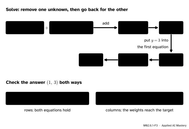
Solve. Add the two equations. On the left, \(x + (-x) = 0\) and \(y + 2y = 3y\). On the right, \(4 + 5 = 9\). So \(3y = 9\) and \(y = 3\). Put \(y = 3\) into the first equation: \(x + 3 = 4\), so \(x = 1\).
M02.6.1-F3
The worked example as a trace. Adding the equations removes \(x\) and gives \(y\). Going back gives \(x\). The answer \((1, 3)\) is then checked in the row picture and in the column picture.
Check by rows.\(1 + 3 = 4\) and \(-1 + {2 \cdot 3} = 5\). Both equations hold, so the point \((1, 3)\) is on both lines.
Check by columns.\({1\,(1, -1)} + {3\,(1, 2)} = {(1 + 3,\; -1 + 6)} = (4, 5)\). One step of the first column and three of the second reach the target.
Check as a map.\(T(1, 3) = {(1 + 3,\; -1 + 2 \cdot 3)} = (4, 5)\).
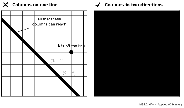
A target that cannot be reached. Change the matrix to \(\begin{bmatrix} 1 & 2 \\ -1 & -2 \end{bmatrix}\) and ask for the target \((3, 0)\) again. The equations are \(x + 2y = 3\) and \(-x - 2y = 0\). Adding them gives \(0 = 3\), which no choice of \(x\) and \(y\) can make true. The column picture shows why. The second column \((2, -2)\) is twice the first, so
a multiple of \((1, -1)\) whatever the weights are. Every reachable output has the form \((s, -s)\). The target \((3, 0)\) does not, so it is outside the span of the columns and the system has no solution.
Code
From scratch first. A solution is checked by multiplying, row by row.
A = [[1, 1], [-1, 2]]def times(A, x):"""A times x, one row at a time."""returntuple(sum(a * xj for a, xj inzip(row, x)) for row in A)def is_solution(A, x, b):return times(A, x) ==tuple(b)print("A times (1, 2) =", times(A, (1, 2)))print("A times (2, 1) =", times(A, (2, 1)))print("is (2, 1) a solution for b = (3, 0)?", is_solution(A, (2, 1), (3, 0)))
A times (1, 2) = (3, 3)
A times (2, 1) = (3, 0)
is (2, 1) a solution for b = (3, 0)? True
Now solve instead of guessing. The function below does what the worked example did: it removes \(x\) from the second equation, finds \(y\), then goes back for \(x\).
def solve_2x2(A, b):"""Solve a 2 by 2 system by removing x from the second equation.""" (a11, a12), (a21, a22) = A b1, b2 = b m = a21 / a11 # how much of equation 1 to take away from equation 2 y = (b2 - m * b1) / (a22 - m * a12) x = (b1 - a12 * y) / a11return (x, y)print("target (3, 0):", solve_2x2(A, (3, 0)))print("target (4, 5):", solve_2x2(A, (4, 5)))
The function divides by two numbers, a11 and a22 - m * a12, so it breaks when either is zero. The next two lessons deal with both cases. NumPy’s solver copes with a zero a11 by reordering the equations. When no single answer exists, as in the second case, it says so. The column picture is one line of NumPy.
import numpy as npA = np.array([[1.0, 1.0], [-1.0, 2.0]])b = np.array([4.0, 5.0])x = np.linalg.solve(A, b)print("solution:", x)print("column check:", x[0] * A[:, 0] + x[1] * A[:, 1])flat = np.array([[1.0, 2.0], [-1.0, -2.0]]) # the second column is twice the firsttry: np.linalg.solve(flat, np.array([3.0, 0.0]))except np.linalg.LinAlgError as error:print("no unique solution:", error)
numpy.linalg.solve refuses the second system because its columns lie along one line, so no target has a single answer. This target, \((3, 0)\), has no answer at all.
Explore
This module’s interactive, the elimination stepper, lives in the next lesson. Its Two lines preset is the row picture of this lesson’s system. Watch for one thing there: the lines turn, but the point where they cross never moves.
Pitfalls
M02.6.1-F4
Wrong beside right. Two columns along one line can only reach the points of that line, so most targets have no solution. Two columns in different directions reach every target in the plane.
“Two equations and two unknowns always have exactly one solution.”
Counting equations is not enough. If the columns lie along one line, a target off that line has no solution, and a target on it has many. This matters in machine learning. Fitting a model with weights \(\vect{w}\) to data means solving \(\mat{X}\vect{w} = \vect{y}\), where each column of \(\mat{X}\) holds one feature. With more data points than features the target \(\vect{y}\) is almost never in the span of the columns, so there is no exact solution. Least squares (lesson M02.10.4) then finds the reachable point nearest to \(\vect{y}\).
“The row picture and the column picture are one drawing seen twice.”
They are drawn in different spaces. The lines of the row picture are sets of inputs. The arrows of the column picture are outputs. For a two-by-two system both spaces happen to be planes, which hides the difference. With three equations in two unknowns, the row picture is three lines in a plane and the column picture is two arrows in three-dimensional space.
“In the column picture, \(x\) and \(y\) are the coordinates of a point on the page.”
There they are weights: how many steps to take along each column. The solution \((2, 1)\) does not appear as a point in the column picture at all. It appears as “2 of this arrow, 1 of that one”.
Check yourself
Recall
1. In \(\mat{A}\vect{x} = \vect{b}\), what is each of the three symbols called, and which one is unknown?
Show answer
\(\mat{A}\) is the coefficient matrix, \(\vect{x}\) is the unknown vector and \(\vect{b}\) is the right-hand side, or target. Only \(\vect{x}\) is unknown.
2. Read as a question about a map, what does \(\mat{A}\vect{x} = \vect{b}\) ask?
Show answer
Which input does the map \(T(\vect{x}) = \mat{A}\vect{x}\) send to the target \(\vect{b}\)?
3. What does the row picture of a two-by-two system show, and where is the solution in it?
Show answer
One line for each equation, drawn in the input plane. The solution is the point that lies on both lines.
4. What does the column picture ask?
Show answer
How much of each column of \(\mat{A}\) must be added together to reach \(\vect{b}\). The solution is the list of weights.
5. In terms of the columns, when does \(\mat{A}\vect{x} = \vect{b}\) have at least one solution?
Show answer
Exactly when \(\vect{b}\) is in the span of the columns of \(\mat{A}\), that is, when \(\vect{b}\) is a linear combination of them.
Exercises
1.★ Write the system \(2x - y = 1\), \(x + 3y = 11\) in the form \(\mat{A}\vect{x} = \vect{b}\). Then check that \((2, 3)\) is a solution, once by rows and once by columns.
By rows: \({2 \cdot 2} - 3 = 1\) and \(2 + {3 \cdot 3} = 11\). Both equations hold.
By columns: \({2\,(2, 1)} + {3\,(-1, 3)} = {(4 - 3,\; 2 + 9)} = (1, 11)\), which is \(\vect{b}\).
2.★★ Find the input that the running map \(T(x, y) = {(x + y,\; -x + 2y)}\) sends to \((0, 3)\). Say what the row picture and the column picture of your answer look like.
Show solution
The system is \(x + y = 0\) and \(-x + 2y = 3\). Adding the equations gives \(3y = 3\), so \(y = 1\). Then \(x + 1 = 0\), so \(x = -1\). The input is \((-1, 1)\). Check: \(T(-1, 1) = {(-1 + 1,\; 1 + 2)} =
(0, 3)\).
Row picture: the line \(x + y = 0\) through the origin and the line \(-x + 2y = 3\) cross at \((-1, 1)\).
Column picture: \(-1\) step of \((1, -1)\), which is one step backwards along the first column, and \(1\) step of \((1, 2)\): \(-(1, -1) + (1, 2) = (0, 3)\).
3.★★★ A matrix has the columns \((1, 2)\) and \((3, 6)\). (a) Describe every target that can be reached. (b) Show that \((2, 4)\) can be reached, and find two different solutions. (c) Can \((1, 0)\) be reached?
Show solution
(a) The second column is 3 times the first, so \({x\,(1, 2)} + {y\,(3, 6)} = {(x + 3y)\,(1, 2)}\). Every reachable target is a multiple of \((1, 2)\): it has the form \((s, 2s)\).
(b) \((2, 4) = 2\,(1, 2)\), so we need \(x + 3y = 2\). Two choices are \((x, y) = (2, 0)\) and \((x, y) = (-1, 1)\). Check the second: \(-(1, 2) + (3, 6) = (2, 4)\). In fact every point of the line \(x + 3y = 2\) is a solution.
(c) No. A target of the form \((s, 2s)\) with first coordinate 1 must be \((1, 2)\), not \((1, 0)\). So \((1, 0)\) is outside the span of the columns and the system has no solution.
This matrix never gives exactly one solution: it gives none or many. Lesson M02.6.3 explains why.
Summary card
A linear system gives the output of a map and asks for the input.
M02.6.1-F1
Find the input that hits the target.
Matrix form. Several linear equations at once are one equation, \(\mat{A}\vect{x} = \vect{b}\).
Row picture. Each row is a line (or a plane) of inputs. Solutions lie on all of them.
Reachable. A solution exists exactly when \(\vect{b}\) is in the span of the columns.
Sources and next steps
Sources. Each was opened and checked against this lesson on 12 November 2026.
Gilbert Strang, The geometry of linear equations, MIT OpenCourseWare 18.06SC, with its lecture summary. The sections “Row Picture”, “Column Picture” and “Matrix Picture” draw one two-by-two system in the ways used here, and the closing section describes the singular case, in which the combinations of the columns do not fill the plane.
Dan Margalit and Joseph Rabinoff, Interactive Linear Algebra, Georgia Institute of Technology (open access). Section 1.1 defines a solution and the solution set. Section 2.3 defines \(\mat{A}\vect{x}\) as a combination of the columns and states, under “Spans and Consistency”, that \(\mat{A}\vect{x} = \vect{b}\) has a solution if and only if \(\vect{b}\) is in the span of the columns.
Grant Sanderson, Inverse matrices, column space and null space, 3Blue1Brown, Linear Algebra, chapter 7. The source of the framing in this lesson: solving \(\mat{A}\vect{x} = \vect{v}\) means looking for the vector that lands on \(\vect{v}\) after the transformation.
Next.M02.6.2 Elimination, step by step turns the “add the two equations” trick of the worked example into a method that solves systems of any size.