The numbers that name a vector are a recipe written for one particular grid. Learn to read the same arrow on a second grid, find its new coordinates by solving two small equations, and see why no single list of numbers is the vector itself.
Explain why the coordinates of a vector are weights on a chosen basis, so that one arrow has different coordinates in different bases.
Read the coordinates of a vector off a slanted grid by sliding along its grid lines.
Find the coordinates of a vector in a new basis of the plane by solving two equations in two unknowns.
Show that taking coordinates respects adding and scaling.
In review. The maths and code on this page are checked by automated tests on every change, but an independent reader has not signed it off yet. Spot a mistake or a confusing step? Tell us.
The question
A camera records a photo as one brightness number for each pixel. A JPEG file holds the same photo as a quite different list of numbers, many of them small enough to throw away. The picture has not changed. What changed is the set of building blocks that the numbers count. So what does a list such as \((1, 5)\) really say about a vector, and how do you rewrite it for a different set of building blocks?
Intuition
The pair \((1, 5)\) is a set of instructions: take 1 step of \(\ihat\), then 5 steps of \(\jhat\). The numbers are the weights in a linear combination, \(1\,\ihat + 5\,\jhat\), and the arrow you end up with is the vector.
Nothing forces us to step along \(\ihat\) and \(\jhat\). Lesson M02.2.4 tried it once: counted in steps of \((1, -1)\) and \((1, 2)\), the point \((5, 1)\) had the coordinates \((3, 2)\). This module turns that one example into a method. Take a fresh pair of building blocks,
They do not lie along one line, so they form a basis of the plane (lesson M02.2.4): every arrow can be reached by stepping along them, in exactly one way. Their whole-number combinations draw a slanted grid. Lay that grid under the same arrow and count again.
M02.9.1-F1
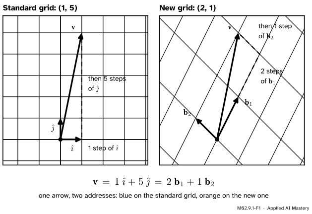
One arrow, two addresses. On the standard grid the arrow \(\vect{v}\) is \((1, 5)\). On the grid of \(\vect{b}_1\) and \(\vect{b}_2\) the same arrow is \((2, 1)\): two steps of \(\vect{b}_1\), then one of \(\vect{b}_2\).
The arrow did not move between the two panels. Only its description changed. Coordinates are not the vector. They are a recipe for the vector, written for one particular basis. Throughout this module, blue marks the standard basis and everything counted on it, and orange marks the new basis and everything counted on that.
Build it up
Step 1. Standard coordinates are weights. Writing \(\vect{v} = (1, 5)\) is short for \(\vect{v} = 1\,\ihat + 5\,\jhat\). The basis is so familiar that we stop mentioning it.
Step 2. A second basis draws a second grid. Call the new basis \(B\): the list \(\vect{b}_1, \vect{b}_2\), in that order. One family of its grid lines runs along \(\vect{b}_1\), the other along \(\vect{b}_2\), and each cell is a copy of the parallelogram the two arrows span.
Step 3. New coordinates are the new weights. The coordinates of \(\vect{v}\) in the basis \(B\) are the two numbers \(c_1, c_2\) with \(\vect{v} = c_1\vect{b}_1 + c_2\vect{b}_2\). We write them as \([\vect{v}]_B = (c_1, c_2)\). The figure shows \([\vect{v}]_B = (2, 1)\).
Step 4. Read them by sliding along the grid. From the tip of the arrow, slide along the \(\vect{b}_2\) grid line until you meet the line through \(\vect{b}_1\). How far along that line you land, counted in copies of \(\vect{b}_1\), is \(c_1\). Sliding the other way gives \(c_2\).
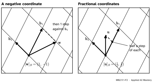
Step 5. Coordinates can be negative or fractions. A negative coordinate means stepping against a basis vector. A fraction means part of a step.
M02.9.1-F2
The arrow \(\vect{w} = (2, 1)\) needs one step of \(\vect{b}_1\) and one step against\(\vect{b}_2\), so \([\vect{w}]_B = (1, -1)\). The arrow \(\vect{u} = (0, 1.5)\) needs half a step of each.
Step 6. One direction is easy, the other is a puzzle. Given new coordinates, finding the arrow is plain arithmetic: \(2\,\vect{b}_1 + 1\,\vect{b}_2 = (2, 4) + (-1, 1) = (1, 5)\). Given the arrow, finding its new coordinates means asking which weights work. That is a small linear system, the kind module M02.6 taught you to solve.
The formal statement
NoteDefinition: coordinates in a basis
Let \(B\) be a basis \(\vect{b}_1, \dots, \vect{b}_n\) of \(\R^n\), listed in a fixed order. The coordinates of \(\vect{v}\) in \(B\) are the numbers \(c_1, \dots, c_n\) for which
The list \([\vect{v}]_B = (c_1, \dots, c_n)\) is the coordinate vector of \(\vect{v}\) in \(B\).
The definition says “the numbers”, and that needs two facts. Such numbers exist, because a basis spans the space. They are the only ones, because a basis is independent: lesson M02.2.4 proved that two different recipes for one vector would give a non-trivial combination equal to \(\vect{0}\).
The ordinary coordinates are the special case where \(B\) is the standard basis, since \((x, y) = x\,\ihat + y\,\jhat\).
Finding the coordinates in the plane. Let \(\vect{b}_1 = (p, r)\), \(\vect{b}_2 = (q, s)\) and \(\vect{v} = (x, y)\). The equation \(c_1\vect{b}_1 + c_2\vect{b}_2 = \vect{v}\), read one coordinate at a time, is two equations:
The new coordinates come out of the standard ones. The number \({ps - qr}\) is the determinant of module M02.8: apart from its sign, the area of one cell of the new grid. It is zero exactly when \(\vect{b}_1\) and \(\vect{b}_2\) lie along one line, and then they are not a basis and there is nothing to divide by.
Taking coordinates respects adding and scaling. Suppose \([\vect{u}]_B = (a_1, a_2)\) and \([\vect{v}]_B = (c_1, c_2)\). Then
That is a recipe for \(\vect{u} + \vect{v}\) in the basis \(B\), and recipes are unique, so \({[\vect{u} + \vect{v}]_B} = [\vect{u}]_B + [\vect{v}]_B\). In the same way, \(k\vect{v} = (kc_1)\vect{b}_1 + (kc_2)\vect{b}_2\), so \([k\vect{v}]_B = k\,[\vect{v}]_B\). These are the two rules of a linear map (lesson M02.4.1). So passing from a vector to its coordinates is a linear map, and the next lesson finds its matrix.
Worked example
Find the coordinates of \(\vect{v} = (1, 5)\) in the basis \(\vect{b}_1 = (1, 2)\), \(\vect{b}_2 = (-1, 1)\).
M02.9.1-F3
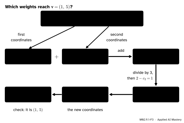
The whole calculation. One vector equation becomes two ordinary equations, adding them removes \(c_2\), and the answer is checked by rebuilding the arrow.
We need \(c_1(1, 2) + c_2(-1, 1) = (1, 5)\). The first coordinates give \(c_1 - c_2 = 1\). The second coordinates give \(2c_1 + c_2 = 5\).
A second vector. For \(\vect{w} = (2, 1)\) the formulas give \(c_1 = \frac{1 \cdot 2 - (-1) \cdot 1}{3} = 1\) and \(c_2 = \frac{1 \cdot 1 - 2 \cdot 2}{3} = -1\), so \([\vect{w}]_B = (1, -1)\), as in the figure above.
Adding survives. The sum \(\vect{v} + \vect{w} = (3, 6)\) should have coordinates \((2, 1) + (1, -1) = (3, 0)\). It does: \(3\,\vect{b}_1 + 0\,\vect{b}_2 = (3, 6)\).
An old example, by the formulas. Lesson M02.2.4 found that \((5, 1)\) has the coordinates \((3, 2)\) in the basis \((1, -1), (1, 2)\). There \(p = 1\), \(r = -1\), \(q = 1\), \(s = 2\), so \({ps - qr} = {1 \cdot 2} - {1 \cdot (-1)} = 3\), and the formulas agree: \(c_1 = \frac{2 \cdot 5 - 1 \cdot 1}{3} = 3\) and \(c_2 = \frac{1 \cdot 1 - (-1) \cdot 5}{3} = 2\).
Code
First from scratch: the two formulas, nothing else.
def coordinates(b1, b2, v):"""The weights (c1, c2) with c1*b1 + c2*b2 == v, from the two formulas.""" (p, r), (q, s), (x, y) = b1, b2, v cell = p * s - q * r # zero exactly when b1, b2 are parallelif cell ==0:raiseValueError("b1 and b2 lie along one line: not a basis")return ((s * x - q * y) / cell, (p * y - r * x) / cell)b1, b2 = (1, 2), (-1, 1)vectors = [("v", (1, 5)), ("w", (2, 1)), ("u", (0, 1.5)), ("v + w", (3, 6))]for name, vec in vectors:print(f"{name:5} = {vec} has coordinates {coordinates(b1, b2, vec)} in B")
v     = (1, 5)  has coordinates (2.0, 1.0) in B
w     = (2, 1)  has coordinates (1.0, -1.0) in B
u     = (0, 1.5)  has coordinates (0.5, 0.5) in B
v + w = (3, 6)  has coordinates (3.0, 0.0) in B
Now the library version. Put the basis vectors side by side as the columns of an array and ask NumPy to solve the system.
import numpy as npB = np.column_stack([b1, b2]) # columns are b1 and b2v = np.array([1.0, 5.0])c = np.linalg.solve(B, v) # solves c[0]*b1 + c[1]*b2 = vprint("coordinates of v in B:", c)print("rebuilt from them: ", c[0] * B[:, 0] + c[1] * B[:, 1])
coordinates of v in B: [2. 1.]
rebuilt from them:     [1. 5.]
np.linalg.solve does by elimination what the worked example did by hand. The hidden cell after it checks, on a hundred random vectors, that coordinates add and scale as the formal section proved.
Explore
This module’s interactive, the two-grid viewer, lives in the next lesson. There you can drag the arrow and the two basis vectors and watch both sets of coordinates change.
Pitfalls
M02.9.1-F4
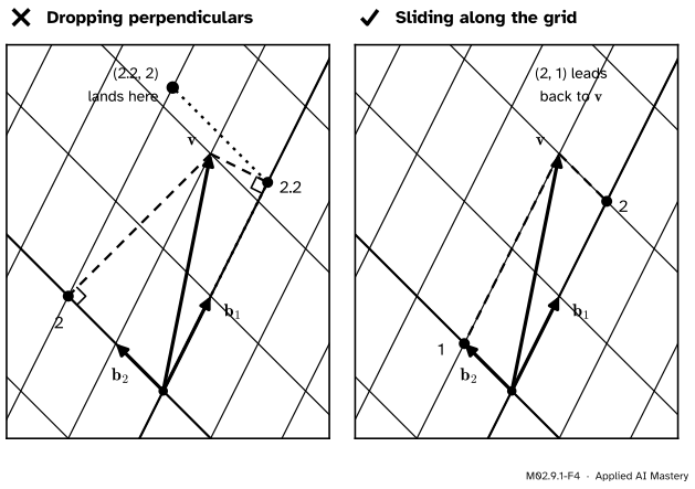
Wrong beside right. On a slanted grid, dropping perpendiculars gives numbers that do not rebuild the arrow. Sliding along the grid lines gives the coordinates.
“To read a coordinate, drop a perpendicular onto the axis.”
That works on the standard grid only because its axes are perpendicular. On the grid of \(\vect{b}_1, \vect{b}_2\) the perpendiculars from \(\vect{v}\) land at \(2.2\) and \(2\), and \(2.2\,\vect{b}_1 + 2\,\vect{b}_2 = (0.2, 6.4)\), which is not \(\vect{v}\). Slide parallel to the other basis vector instead. The shortcut is safe only when the basis vectors are perpendicular to each other, and module M02.10 shows why it works then.
“The vector is its list of numbers.”
The numbers mean nothing until you say which basis they count. The pair \((2, 1)\) names the arrow \((2, 1)\) on the standard grid and the arrow \((1, 5)\) on the grid of \(B\). This matters throughout machine learning: the features of a data set are coordinates in a basis that somebody chose, and methods such as principal component analysis start by choosing a better one.
“In the basis \(B\), the vector \(\vect{b}_1\) still has coordinates \((1, 2)\).”
\((1, 2)\) is its standard address. In its own basis, \(\vect{b}_1 = 1\,\vect{b}_1 + 0\,\vect{b}_2\), so \([\vect{b}_1]_B = (1, 0)\), and likewise \([\vect{b}_2]_B = (0, 1)\). Every basis looks like the standard basis to itself.
Check yourself
Recall
1. What do the coordinates of a vector in a basis \(B\) tell you?
Show answer
The weights of the one linear combination of the basis vectors that equals the vector: \([\vect{v}]_B = (c_1, c_2)\) means \(\vect{v} = c_1\vect{b}_1 + c_2\vect{b}_2\).
2. Why does every vector have exactly one set of coordinates in a basis?
Show answer
A basis spans the space, so at least one recipe exists. A basis is independent, so two different recipes for one vector are impossible.
3. On a slanted grid, how do you read the \(\vect{b}_1\) coordinate of an arrow from the picture?
Show answer
Slide from the tip parallel to \(\vect{b}_2\) until you meet the line through \(\vect{b}_1\), then count how many copies of \(\vect{b}_1\) reach that point. Do not drop a perpendicular.
4. What are the coordinates of \(\vect{b}_2\) in the basis \(\vect{b}_1, \vect{b}_2\)?
Show answer
\((0, 1)\), because \(\vect{b}_2 = 0\,\vect{b}_1 + 1\,\vect{b}_2\).
5. Which direction needs a system of equations: from new coordinates to the arrow, or from the arrow to new coordinates?
Show answer
From the arrow to its new coordinates. The other direction is just computing \(c_1\vect{b}_1 + c_2\vect{b}_2\).
Exercises
1.★ Find the coordinates of \((3, 3)\) in the basis \(\vect{b}_1 = (1, 2)\), \(\vect{b}_2 = (-1, 1)\), and check your answer.
Show solution
The equations are \(c_1 - c_2 = 3\) and \(2c_1 + c_2 = 3\). Adding them gives \(3c_1 = 6\), so \(c_1 = 2\), and then \(2 - c_2 = 3\) gives \(c_2 = -1\). The coordinates are \((2, -1)\). Check: \(2\,(1, 2) - 1\,(-1, 1) = {(2 + 1,\; 4 - 1)} = (3, 3)\).
2.★★ A vector has \([\vect{x}]_B = (-1, 2)\) in the same basis \(B\). (a) What is \(\vect{x}\) in standard coordinates? (b) What are its coordinates if the basis vectors are listed in the other order, \(\vect{b}_2, \vect{b}_1\)? (c) What are they in the basis \(2\vect{b}_1, \vect{b}_2\)?
(b) The recipe is the same, \(\vect{x} = 2\,\vect{b}_2 + (-1)\,\vect{b}_1\), but the weights are now listed in the new order: \((2, -1)\). This is why a basis is an ordered list.
(c) Write \(-1\,\vect{b}_1\) as \(-\tfrac12\,(2\vect{b}_1)\). Then \(\vect{x} = -\tfrac12\,(2\vect{b}_1) + 2\,\vect{b}_2\), so the coordinates are \((-\tfrac12, 2)\). Doubling a basis vector halves the coordinate that counts it.
3.★★★ Let \(\vect{b}_1, \vect{b}_2\) be any basis of the plane and let \([\vect{v}]_B = (c_1, c_2)\). Show that \(\vect{b}_1 + \vect{b}_2,\ \vect{b}_2\) is also a basis, and that the coordinates of \(\vect{v}\) in it are \({(c_1,\; c_2 - c_1)}\).
Show solution
It is a basis. Two vectors form a basis of the plane when they are independent. Suppose \(\alpha{(\vect{b}_1 + \vect{b}_2)} + \beta\,\vect{b}_2 = \vect{0}\). Regrouping, \(\alpha\,\vect{b}_1 + {(\alpha + \beta)}\,\vect{b}_2 = \vect{0}\). Because \(\vect{b}_1, \vect{b}_2\) are independent, \(\alpha = 0\) and \(\alpha + \beta = 0\), so \(\beta = 0\) too. Only the trivial combination gives zero.
The coordinates. Start from the old recipe and regroup:
The right-hand side is a recipe in the new basis, and recipes are unique, so the coordinates are \({(c_1,\; c_2 - c_1)}\). With this lesson’s numbers, \((2, 1)\) becomes \((2, -1)\), and indeed \(2\,(0, 3) - 1\,(-1, 1) = (1, 5)\).
Summary card
Coordinates are a recipe for a vector, written for one basis.
M02.9.1-F1
One arrow, two addresses.
Definition.\([\vect{v}]_B = (c_1, c_2)\) means \(\vect{v} = c_1\vect{b}_1 + c_2\vect{b}_2\).
Finding them. Solve \(c_1\vect{b}_1 + c_2\vect{b}_2 = \vect{v}\): two equations, two unknowns.
In the plane. With \(\vect{b}_1 = (p, r)\), \(\vect{b}_2 = (q, s)\): \(c_1 = \dfrac{sx - qy}{ps - qr}\), \(c_2 = \dfrac{py - rx}{ps - qr}\).
Sources. Each was opened and checked against this lesson on 12 November 2026.
Dan Margalit and Joseph Rabinoff, Interactive Linear Algebra, Section 2.8, Bases as Coordinate Systems (open textbook, Georgia Tech). It states that a vector is a combination of basis vectors in exactly one way, defines the \(B\)-coordinates and the notation \([\vect{x}]_B\) used here, and finds them by solving the vector equation.
Grant Sanderson, Change of basis, 3Blue1Brown, Linear Algebra, chapter 13. The source of the two-grids picture: a second person whose basis vectors are \((2, 1)\) and \((-1, 1)\) describes the same vectors with different numbers.
Gilbert Strang, Change of basis; image compression, MIT OpenCourseWare 18.06SC, lecture 31. The lecture summary describes JPEG compression as a change from the pixel basis to a basis of cosines on blocks of 8 by 8 pixels, after which many coefficients are small enough to drop.
NumPy reference, numpy.linalg.solve. Solves a full-rank square system \(ax = b\), and raises LinAlgError if \(a\) is singular.
Next.M02.9.2 The change-of-basis matrix packs the two equations into one matrix, so that converting a vector, or a million of them, is a single multiplication.