Every row operation is multiplication by a matrix, and elimination as a whole is the factorisation A = LU. See why the multipliers drop straight into L, solve with two triangular systems, count the work, and learn why numerical code calls solve and does not form an inverse.
Write the matrix that performs a given row operation, and the matrix that undoes it.
Explain why forward elimination without row swaps factorises a matrix as A = LU, with the multipliers as the entries of L.
Solve a system from its factors L and U by forward and back substitution.
Estimate how the work of elimination and of substitution grows with the number of unknowns.
Explain why numerical code solves a system directly and does not form the inverse.
In review. The maths and code on this page are checked by automated tests on every change, but an independent reader has not signed it off yet. Spot a mistake or a confusing step? Tell us.
The question
numpy.linalg.solve handles a system with a thousand unknowns in a fraction of a second, and machine-learning libraries lean on such routines constantly. Inside, nobody shuffles equations. The routine factorises a matrix. How can “take twice row 1 from row 2” be a matrix, and what is gained by seeing elimination that way?
From the last lesson
1. After elimination, which kind of row shows that there is no solution?
Show answer
A row with zeros before the bar and a non-zero number after it. It says \(0 = c\) with \(c \neq 0\).
2. What is a free variable?
Show answer
An unknown whose column has no pivot in the echelon form. It can be given any value.
Intuition
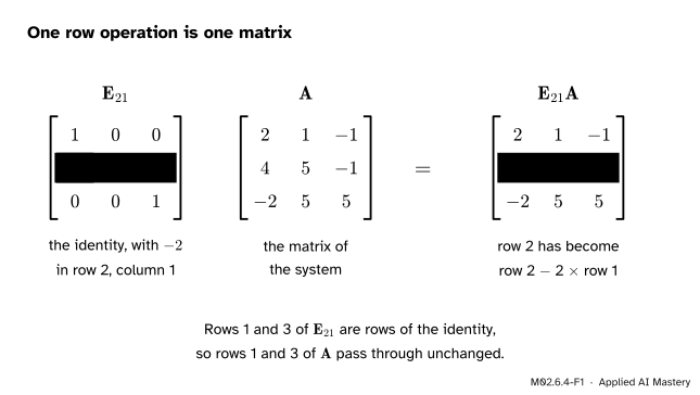
A row operation rewrites the rows of a matrix. So does multiplying on the left by another matrix. For each row operation there is a matrix that does the same job, and a recipe finds it: do the operation to the identity matrix. What comes out does that operation to anything it multiplies.
Take the first step of the worked example in lesson M02.6.2, \({R_2 \leftarrow R_2 - 2R_1}\). Applied to the identity it changes row 2 from \((0, 1, 0)\) to \((-2, 1, 0)\). Call the result \(\mat{E}_{21}\), after the position of the entry it clears.
M02.6.4-F1
\(\mat{E}_{21}\) is the identity with one extra entry. Multiplying by it takes twice row 1 from row 2 and leaves the rest alone.
The recipe works because each row of a product \(\mat{E}\mat{A}\) is a combination of the rows of \(\mat{A}\), with weights read from the matching row of \(\mat{E}\). Row 2 of \(\mat{E}_{21}\) is \((-2, 1, 0)\): take \(-2\) of row 1 and 1 of row 2.
Build it up
Step 1. Rows of a product. By the multiplication rule of lesson M02.5.2, the entry of \(\mat{E}\mat{A}\) in row \(i\) and column \(j\) is \(e_{i1}a_{1j} + e_{i2}a_{2j} + e_{i3}a_{3j}\). Keep \(i\) fixed and let \(j\) run along the row. The same three weights \(e_{i1}, e_{i2}, e_{i3}\) appear in every entry, so
\[
\begin{aligned}
&\text{row } i \text{ of } \mat{E}\mat{A} \\
&\quad = e_{i1}\,(\text{row 1 of } \mat{A}) \\
&\qquad {} + e_{i2}\,(\text{row 2 of } \mat{A}) \\
&\qquad {} + e_{i3}\,(\text{row 3 of } \mat{A}).
\end{aligned}
\]
Step 2. Three steps, three matrices. The worked example used three operations. Each one has its matrix:
They perform \({R_2 \leftarrow R_2 - 2R_1}\), then \({R_3 \leftarrow R_3 + R_1}\), then \({R_3 \leftarrow R_3 - 2R_2}\). Applied one after another they turn \(\mat{A}\) into the triangular matrix \(\mat{U}\):
The first operation sits nearest to \(\mat{A}\), because the map applied first is written on the right (lesson M02.5.1).
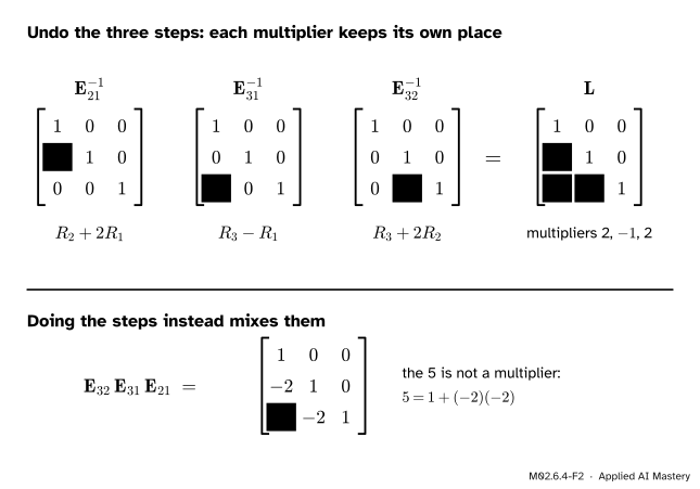
Step 3. Undo a step. To undo “take 2 times row 1 from row 2”, add it back. The matrix that adds 2 times row 1 to row 2 is the identity with \(+2\) in the same position. We write it \(\mat{E}_{21}^{-1}\) and call it the inverse of \(\mat{E}_{21}\): applying one and then the other changes nothing, so their product is the identity.
Step 4. Move the steps to the other side. Undo the three steps, last one first, on both sides of the equation in Step 2. On the left only \(\mat{A}\) remains:
Multiply the three undo matrices together and the multipliers 2, \(-1\) and 2 drop into place.
M02.6.4-F2
The product of the undo matrices is \(\mat{L}\), with each multiplier where it was used. The product that does the steps is less tidy: its corner entry 5 mixes two multipliers.
So \(\mat{A} = \mat{L}\mat{U}\): a lower triangular matrix \(\mat{L}\) that records the steps of elimination, times the upper triangular matrix \(\mat{U}\) that elimination produced.
The formal statement
NoteDefinition: elementary matrix
An elementary matrix is the result of applying one row operation to the identity matrix. For \(i \neq j\), write \(\mat{E}_{ij}(c)\) for the identity with one extra entry \(c\) in row \(i\), column \(j\).
Claim 1: \(\mat{E}_{ij}(c)\,\mat{A}\) is \(\mat{A}\) with \(c\) times row \(j\) added to row \(i\). Use the row rule of Step 1, which holds for any number of rows. For \(k \neq i\), row \(k\) of \(\mat{E}_{ij}(c)\) is row \(k\) of the identity: a single 1 in position \(k\). So row \(k\) of the product is 1 times row \(k\) of \(\mat{A}\), unchanged. Row \(i\) of \(\mat{E}_{ij}(c)\) has a 1 in position \(i\) and \(c\) in position \(j\). So row \(i\) of the product is (row \(i\) of \(\mat{A}\)) plus \(c\) times (row \(j\) of \(\mat{A}\)). The matrices for a swap and for a scaling are checked in the same way.
Claim 2: \(\mat{E}_{ij}(-c)\) undoes \(\mat{E}_{ij}(c)\). A matrix \(\mat{B}\) is the inverse of \(\mat{A}\), written \(\mat{A}^{-1}\), if \(\mat{B}\mat{A} = \mat{I}\) and \(\mat{A}\mat{B} = \mat{I}\). (Lesson M02.7.1 studies which matrices have one.) By Claim 1, \(\mat{E}_{ij}(-c)\,\mat{E}_{ij}(c)\) is \(\mat{E}_{ij}(c)\) with \(-c\) times its row \(j\) added to its row \(i\). Its row \(j\) is row \(j\) of the identity. Its row \(i\) is (row \(i\) of the identity) plus \(c\) times (row \(j\) of the identity). The sum is
\[
\begin{aligned}
&(\text{row } i \text{ of } \mat{I}) + c\,(\text{row } j \text{ of } \mat{I}) \\
&\quad {} - c\,(\text{row } j \text{ of } \mat{I})
= \text{row } i \text{ of } \mat{I},
\end{aligned}
\]
so the product is the identity. Exchanging \(c\) and \(-c\) gives the product in the other order. Hence \(\mat{E}_{ij}(c)^{-1} = \mat{E}_{ij}(-c)\).
NoteResult: A = LU
Suppose forward elimination on a square matrix \(\mat{A}\) needs no row swaps. Let \(\mat{U}\) be the upper triangular matrix it produces, and let \(m_{ik}\) be the multiplier used to clear the entry in row \(i\), column \(k\). Then \(\mat{A} = \mat{L}\mat{U}\), where \(\mat{L}\) is lower triangular with ones on its diagonal and \(m_{ik}\) in row \(i\), column \(k\).
Derivation, three by three. Clearing an entry with multiplier \(m_{ik}\) is the operation \({R_i \leftarrow R_i - m_{ik}R_k}\), so its matrix is \(\mat{E}_{ik}(-m_{ik})\). Write \(\mat{E}_{21}\), \(\mat{E}_{31}\), \(\mat{E}_{32}\) for the three of them. Elimination says
Multiply both sides on the left by \(\mat{E}_{32}^{-1}\). On the left \(\mat{E}_{32}^{-1}\mat{E}_{32} = \mat{I}\) disappears: \(\mat{E}_{31}\mat{E}_{21}\mat{A} = \mat{E}_{32}^{-1}\mat{U}\). Do the same with \(\mat{E}_{31}^{-1}\): \(\mat{E}_{21}\mat{A} = \mat{E}_{31}^{-1}\mat{E}_{32}^{-1}\mat{U}\). And with \(\mat{E}_{21}^{-1}\):
Now compute \(\mat{L}\) from right to left. By Claim 2, each inverse is the identity with \(+m\) in place of \(-m\), and by Claim 1, multiplying by it on the left adds a multiple of one row to another. Start with \(\mat{E}_{32}^{-1}\). Multiplying it on the left by \(\mat{E}_{31}^{-1}\) adds \(m_{31}\) times its row 1 to its row 3. Row 1 is \((1, 0, 0)\), so only the first entry of row 3 changes:
Multiplying that on the left by \(\mat{E}_{21}^{-1}\) adds \(m_{21}\) times row 1 to row 2. Row 1 is still \((1, 0, 0)\), so only the first entry of row 2 changes:
Each multiplier lands in its own position, because the row being added carries nothing else with it. In the worked example \(m_{21} = 2\), \(m_{31} = -1\) and \(m_{32} = 2\). The same argument, one column at a time, works for any size.
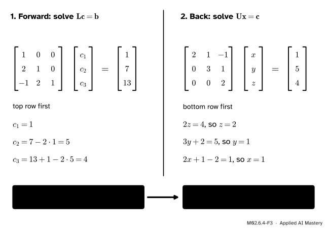
Solving with the factors. Since \(\mat{A} = \mat{L}\mat{U}\), the system \(\mat{A}\vect{x} = \vect{b}\) is \(\mat{L}(\mat{U}\vect{x}) = \vect{b}\). Name the inner vector \(\vect{c} = \mat{U}\vect{x}\) and solve two triangular systems:
\(\mat{L}\vect{c} = \vect{b}\), from the top row down. This is forward substitution.
\(\mat{U}\vect{x} = \vect{c}\), from the bottom row up. This is back substitution.
Forward substitution replays on \(\vect{b}\) the row operations that elimination applied to \(\mat{A}\). Its result \(\vect{c}\) is the last column of the triangular augmented matrix of lesson M02.6.2.
When rows must be swapped. A swap is an elementary matrix too: the identity with two rows exchanged. If elimination needs swaps, do them all first. The reordered matrix \(\mat{P}\mat{A}\), where \(\mat{P}\) is the identity with its rows reordered, then factorises as \(\mat{P}\mat{A} = \mat{L}\mat{U}\). At every step libraries swap the entry of largest absolute value in the column into the pivot position. This keeps rounding errors small and is called partial pivoting.
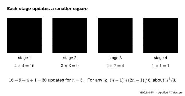
A first look at the cost. Count the updates “entry minus multiplier times entry”. At stage \(k\) there are \(n - k\) rows below the pivot, and in each of them the \(n - k\) entries to the right of the pivot column are updated. So stage \(k\) costs \({(n - k)}^2\) updates.
M02.6.4-F4
Forward elimination on a five-by-five matrix. Yellow is the pivot and green are the entries updated at that stage. The green squares shrink, and their sizes add up to the cost.
Adding the stages, and using the formula \(1^2 + 2^2 + \cdots + N^2 = \tfrac16 N{(N + 1)}{(2N + 1)}\) with \(N = n - 1\),
One forward and one back substitution together cost exactly \(n^2\) operations. Row \(i\) of \(\mat{L}\) uses \(i - 1\) earlier values, row \(i\) of \(\mat{U}\) uses \(n - i\) later values, and back substitution adds \(n\) divisions by the pivots: \(\tfrac12 n{(n-1)} + \tfrac12 n{(n-1)} + n = n^2\). For \(n = 1000\) that is about a third of a billion updates to factorise and a million operations for each right-hand side. Doubling \(n\) multiplies the factorising work by about 8 and the substitution work by 4.
Worked example
Factorise once, solve twice. Take the matrix of lesson M02.6.2. Its multipliers were 2, \(-1\) and 2, and its triangular form is known, so
Now the factorisation itself, and the two substitutions. The only change from the elimination code of lesson M02.6.2 is one line: each multiplier is stored in \(\mat{L}\).
def lu_no_swaps(A):"""Factorise A = L U by forward elimination. Assumes that no zero pivot turns up.""" n =len(A) U = np.array(A, dtype=float) L = np.eye(n)for k inrange(n -1):for i inrange(k +1, n): L[i, k] = U[i, k] / U[k, k] # the multiplier goes straight into L U[i] = U[i] - L[i, k] * U[k]return L, Udef forward_substitute(L, b): c = np.zeros(len(b))for i inrange(len(b)): # the top row first c[i] = b[i] -sum(L[i, j] * c[j] for j inrange(i))return cdef back_substitute(U, c): n =len(c) x = np.zeros(n)for i inrange(n -1, -1, -1): # the bottom row first x[i] = (c[i] -sum(U[i, j] * x[j] for j inrange(i +1, n))) / U[i, i]return xL, U = lu_no_swaps(A)print(L)for b in ([3, 5, -1], [1, 7, 13]): c = forward_substitute(L, b)print("b =", b, " c =", c, " x =", back_substitute(U, c))
[[ 1.  0.  0.]
 [ 2.  1.  0.]
 [-1.  2.  1.]]
b = [3, 5, -1]  c = [ 3. -1.  4.]  x = [ 3. -1.  2.]
b = [1, 7, 13]  c = [1. 5. 4.]  x = [1. 1. 2.]
The library versions. scipy.linalg.lu returns the factors, lu_factor with lu_solve factorises once and solves many times, and numpy.linalg.solve does everything in one call.
The library’s factors are not ours. It swapped rows to put the 4, the largest entry of the first column, in the pivot position, so its \(\mat{U}\) starts with the row \((4, 5, -1)\). The answers agree, because \(\mat{P}\mat{L}\mat{U}\) is still \(\mat{A}\). SciPy’s \(\mat{P}\) puts the rows back in order: it is the inverse of the \(\mat{P}\) in \(\mat{P}\mat{A} = \mat{L}\mat{U}\).
Now count the work, by running the loops.
def count_updates(n):"""Entry updates in forward elimination on an n by n matrix.""" count =0for k inrange(n -1):for i inrange(k +1, n):for j inrange(k +1, n): count +=1return countdef count_substitutions(n):"""Operations in one forward and one back substitution.""" forward =sum(i for i inrange(n)) # row i uses the i values found before it back =sum(n -1- i for i inrange(n)) + n # the later values, then one division per rowreturn forward + backfor n in (3, 5, 100):print(n, count_updates(n), (n -1) * n * (2* n -1) //6, round(n **3/3), count_substitutions(n))n =100solve_cost = count_updates(n) + count_substitutions(n)inverse_cost = count_updates(n) + n * count_substitutions(n) + n * nprint("solve:", solve_cost, " inverse, then multiply:", inverse_cost, " ratio:", round(inverse_cost / solve_cost, 2))
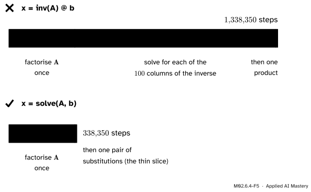
The last line compares two ways to solve one system with 100 unknowns. Finding the inverse by solving for its 100 columns one at a time and then multiplying by \(\vect{b}\) costs about four times as much as solving directly.
Speed is not the only issue. The eight-by-eight Hilbert matrix, with entry \(1/{(i + j - 1)}\) in row \(i\), column \(j\), is hard on rounding errors. We build a system whose true solution is all ones, solve it both ways, and measure how far \(\mat{A}\vect{x}\) is from \(\vect{b}\).
from scipy.linalg import hilbertH = hilbert(8)b = H @ np.ones(8)x_solve = np.linalg.solve(H, b)x_inverse = np.linalg.inv(H) @ bmiss_solve = np.linalg.norm(H @ x_solve - b)miss_inverse = np.linalg.norm(H @ x_inverse - b)print(f"solve: misses b by {miss_solve:.1e}")print(f"inverse: misses b by {miss_inverse:.1e}")
solve:   misses b by 5.6e-16
inverse: misses b by 5.7e-08
On this matrix the answer that came through the inverse misses the target by many orders of magnitude more than the answer from solve. The two printed misses depend on rounding inside the linear-algebra library, so they vary a little from one computer to another. That gap of many orders of magnitude does not.
Explore
The elimination stepper in lesson M02.6.2 names the multiplier at each step of forward elimination. Press Lesson system and step three times, noting the multipliers: 2, then \(-1\), then 2. They are the entries of \(\mat{L}\) below its diagonal.
Pitfalls
M02.6.4-F5
Wrong beside right, for one system with 100 unknowns. Forming the inverse repeats the substitutions a hundred times.
The formula \(\vect{x} = \mat{A}^{-1}\vect{b}\) is true, but it is a poor way to compute. Finding the inverse means solving a system for each of its columns, so it costs several times as much as solving the one system, and the answer is usually less accurate. Call numpy.linalg.solve(A, b). If one matrix meets many right-hand sides, factorise it once with lu_factor and reuse the factors. Linear regression, Gaussian processes and second-order optimisers all contain a step of this kind.
“My \(\mat{L}\) and \(\mat{U}\) differ from the library’s, so one of us is wrong.”
Libraries swap rows for accuracy, and a different row order gives different factors. Check the product \(\mat{P}\mat{L}\mat{U}\), not the factors. Some matrices cannot be factorised at all without a swap, as exercise 3 shows.
Check yourself
Recall
1. How do you find the matrix that performs a given row operation?
Show answer
Apply the operation to the identity matrix. Multiplying on the left by the result applies the operation to any matrix.
2. In \(\mat{E}_{32}\mat{E}_{31}\mat{E}_{21}\mat{A} = \mat{U}\), which operation is applied first?
Show answer
\(\mat{E}_{21}\), the one nearest to \(\mat{A}\).
3. What undoes “take 2 times row 1 from row 2”, and what is its matrix?
Show answer
Adding 2 times row 1 to row 2. Its matrix is the identity with \(+2\) in row 2, column 1.
4. In \(\mat{A} = \mat{L}\mat{U}\), what are \(\mat{L}\) and \(\mat{U}\)?
Show answer
\(\mat{U}\) is the upper triangular matrix that forward elimination produces. \(\mat{L}\) is lower triangular with ones on the diagonal and the multipliers below it, each where it was used.
5. Roughly how does the work grow with the number of unknowns \(n\), for factorising and for one pair of substitutions?
Show answer
Factorising takes about \(n^3/3\) updates. A forward and a back substitution together take \(n^2\) operations.
Exercises
1.★ Write the matrix that adds 3 times row 1 to row 3 of any matrix with three rows. Write its inverse, and check that their product is the identity.
The inverse takes 3 times row 1 away again. Rows 1 and 2 of \(\mat{E}^{-1}\mat{E}\) are rows 1 and 2 of \(\mat{E}\), which are rows of the identity. Row 3 is \(-3\,(1, 0, 0) + 1\,(3, 0, 1) = (0, 0, 1)\). So the product is the identity.
2.★★ Factorise \(\mat{A} = \begin{bmatrix} 3 & 1 \\ 6 & 4 \end{bmatrix}\) as \(\mat{L}\mat{U}\). Then solve \(\mat{A}\vect{x} = (5, 14)\) with a forward and a back substitution.
Show solution
The pivot is 3 and the multiplier is \(6/3 = 2\). \({R_2 \leftarrow R_2 - 2R_1}\) gives the row \((0, 2)\). So
Back, \(\mat{U}\vect{x} = (5, 4)\): \(2y = 4\), so \(y = 2\). Then \(3x + 2 = 5\), so \(x = 1\).
Check: \(3 + 2 = 5\) and \(6 + 8 = 14\).
3.★★★ Show that \(\begin{bmatrix} 0 & 1 \\ 1 & 0 \end{bmatrix}\) cannot be written as \(\mat{L}\mat{U}\) with \(\mat{L}\) lower triangular with ones on its diagonal and \(\mat{U}\) upper triangular. Then show that swapping its rows first removes the difficulty.
Show solution
Suppose it could. Write \(\mat{L} = \begin{bmatrix} 1 & 0 \\ l & 1 \end{bmatrix}\) and \(\mat{U} = \begin{bmatrix} u_{11} & u_{12} \\ 0 & u_{22} \end{bmatrix}\). Their product is
Matching the top-left entry gives \(u_{11} = 0\). Matching the bottom-left entry gives \(l\,u_{11} = 1\), that is, \(l \cdot 0 = 1\). No number \(l\) does that, so no such factors exist.
Swapping the two rows turns the matrix into the identity, which factorises as \(\mat{I} = \mat{I}\,\mat{I}\). With \(\mat{P}\) the matrix of the swap, \(\mat{P}\mat{A} = \mat{L}\mat{U}\) holds with \(\mat{L} = \mat{U} = \mat{I}\).
Summary card
Elimination is matrix multiplication, and it factorises A as LU.
M02.6.4-F1
One row operation, one matrix.
Elementary matrix. Do the row operation to \(\mat{I}\). To undo it, flip the sign of the multiplier.
Factorisation. No swaps needed: \(\mat{A} = \mat{L}\mat{U}\), with the multipliers in \(\mat{L}\). With swaps: \(\mat{P}\mat{A} = \mat{L}\mat{U}\).
Solving.\(\mat{L}\vect{c} = \vect{b}\) from the top, then \(\mat{U}\vect{x} = \vect{c}\) from the bottom.
Cost. About \(n^3/3\) to factorise, \(n^2\) for each right-hand side.
In code.numpy.linalg.solve(A, b), not inv(A) @ b.
Sources and next steps
Sources. Each was opened and checked against this lesson on 12 November 2026.
Gilbert Strang, Factorization into A = LU, MIT OpenCourseWare 18.06SC, with its lecture summary. “A = LU” cancels the elimination matrices, shows a product of them with an unwanted mixed entry, and states that without row exchanges the multipliers are copied directly into \(\mat{L}\). “How expensive is elimination?” gives the count \(\tfrac13 n^3\), and about \(n^2\) for the right-hand side. “Row exchanges” introduces permutation matrices.
NumPy, numpy.linalg.solve, reference for version 2.5. Its notes say the solutions are computed with LAPACK’s _gesv.
LAPACK, DGESV, reference for version 3.12.1. The routine factorises \(\mat{A} = \mat{P}\mat{L}\mat{U}\) with partial pivoting and row interchanges, then solves with the factors.
SciPy, scipy.linalg.lu, reference for version 1.18. LU decomposition with partial pivoting, \(\mat{A} = \mat{P}\mat{L}\mat{U}\), with a unit diagonal in \(\mat{L}\).
Nick Higham, Seven Sins of Numerical Linear Algebra, 11 October 2022. The first sin is inverting a matrix: solving by LU factorisation with partial pivoting is faster and more accurate.
Next. Module M02.7 starts with M02.7.1 The inverse: undoing a map, which asks exactly when a matrix can be undone, and what its inverse looks like when it can.