Shear then turn is not turn then shear, so AB and BA are usually different matrices. See why, then prove what does survive from ordinary arithmetic: brackets can move, and multiplication distributes over addition. A map of which school-algebra habits are safe with matrices.
Show with a rotation and a shear that AB and BA can be different, in pictures and by computing both products.
Prove that matrix multiplication is associative by thinking of the matrices as maps applied in turn.
Prove that matrix multiplication distributes over addition, on both sides.
Sort the rules of ordinary multiplication into those that carry over to matrices and those that fail, with a counterexample for each failure.
In review. The maths and code on this page are checked by automated tests on every change, but an independent reader has not signed it off yet. Spot a mistake or a confusing step? Tell us.
The question
Socks, then shoes. Now try shoes, then socks. With numbers you never have to think about order: \(3 \times 5\) and \(5 \times 3\) are the same. Training a neural network means doing algebra with long products of matrices. Do matrices allow the same freedom as numbers? If not, which habits of school algebra are still safe, and which will quietly give wrong answers?
From the last lesson
1. What are the columns of the product \(\mat{A}\mat{B}\)?
Show answer
\(\mat{A}\) applied to the columns of \(\mat{B}\): column \(j\) of \(\mat{A}\mat{B}\) is \(\mat{A}\vect{b}_j\).
2. How is the entry of \(\mat{A}\mat{B}\) in row \(i\) and column \(j\) computed?
Show answer
Take row \(i\) of \(\mat{A}\) and column \(j\) of \(\mat{B}\), multiply matching entries and add: \(a_{i1}b_{1j} + a_{i2}b_{2j} + \cdots + a_{in}b_{nj}\).
Intuition
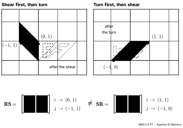
A product of matrices is one map after another, and doing things in a different order usually gives a different result. Take the shear \(\mat{S}\) and the quarter turn \(\mat{R}\) of this module and apply them in both orders.
M02.5.3-F1
The same two maps in the two possible orders. The letter F ends in a different place, so \(\mat{R}\mat{S}\) and \(\mat{S}\mat{R}\) are different maps and different matrices.
Why should the order matter? The shear slides each point sideways by an amount equal to its height. The turn changes heights. Shear first, and \(\jhat\) slides while it is still at height 1. Turn first, and \(\jhat\) is lying on the horizontal axis, at height 0, when the shear arrives: it does not slide at all. One map changes the very thing the other map depends on.
Build it up
Step 1. Both orders, by following the basis vectors. Lesson M02.5.1 found the columns of \(\mat{R}\mat{S}\), shear first: \(\ihat \to (1, 0) \to (0, 1)\) and \(\jhat \to (1, 1) \to (-1, 1)\). Now turn first: \(\ihat \to (0, 1) \to (1, 1)\), because the shear slides a point at height 1 by one unit. And \(\jhat \to (-1, 0) \to (-1, 0)\), because the shear leaves the horizontal axis alone.
Step 2. One difference is enough. Two matrices are equal only if every entry agrees. These differ in the top left corner, so \(\mat{R}\mat{S} \neq \mat{S}\mat{R}\). As maps, they send \(\ihat\) to different places.
Step 3. Some pairs do agree. Two maps commute if the order does not matter: \(\mat{A}\mat{B} = \mat{B}\mat{A}\). Two rotations commute, since turning by \(30°\) and then \(60°\) is the same as turning by \(60°\) and then \(30°\). Two stretches along the axes commute. Every matrix commutes with itself. So the rule is “the order can matter”, and for most pairs it does.
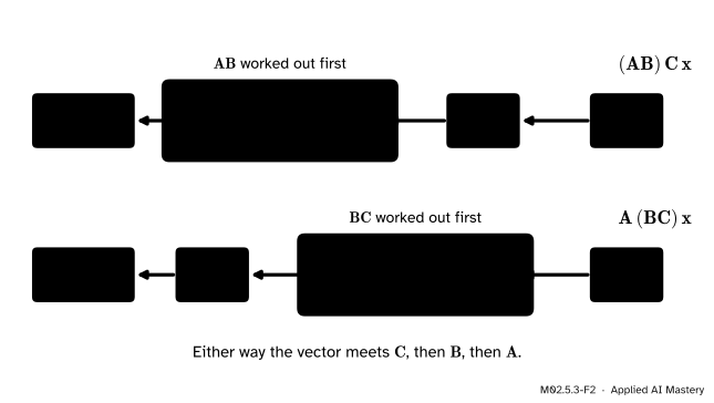
Step 4. Brackets are different: they never matter. Take three maps and write \(\mat{A}\mat{B}\mat{C}\). A vector meets \(\mat{C}\) first, then \(\mat{B}\), then \(\mat{A}\). Brackets do not change that sequence. They only say which two neighbours you multiplied together first on paper.
M02.5.3-F2
Moving the brackets changes which two matrices are merged into one. It does not change the order in which a vector meets the three maps.
Step 5. Maps can be added, and multiplication spreads over the sum. Adding two matrices means adding matching entries. The sum \(\mat{B} + \mat{C}\) is the map that applies both to the same input and adds the outputs: \(\vect{v} \mapsto \mat{B}\vect{v} + \mat{C}\vect{v}\). Follow that with a third map \(\mat{A}\), and its linearity lets it act on the two parts separately: \(\mat{A}(\mat{B} + \mat{C}) = \mat{A}\mat{B} + \mat{A}\mat{C}\).
The formal statement
NoteDefinition: sum and scalar multiple
For matrices \(\mat{B}\) and \(\mat{C}\) of the same shape, \(\mat{B} + \mat{C}\) is the matrix whose entries are the sums of the matching entries, and \(s\,\mat{B}\) is the matrix with every entry of \(\mat{B}\) multiplied by the number \(s\). Their columns are \(\vect{b}_j + \vect{c}_j\) and \(s\,\vect{b}_j\).
As maps: \((\mat{B} + \mat{C})\vect{v} = \mat{B}\vect{v} + \mat{C}\vect{v}\) and \((s\,\mat{B})\vect{v} = s\,(\mat{B}\vect{v})\). For the sum, use the column view with \(\vect{v} = (v_1, \dots, v_p)\):
The second step multiplies out and regroups. The scalar multiple works the same way, with \(s\,\vect{b}_j\) in place of \(\vect{b}_j + \vect{c}_j\).
NoteResult 1: multiplication is associative
Whenever the shapes fit, \((\mat{A}\mat{B})\mat{C} = \mat{A}(\mat{B}\mat{C})\).
Proof. Lesson M02.5.2 showed that a product does both of its steps: \((\mat{P}\mat{Q})\vect{x} = \mat{P}(\mat{Q}\vect{x})\). Apply each side of the claim to any vector \(\vect{x}\) and use that fact twice.
Both sides send every \(\vect{x}\) to the same place: \(\mat{C}\), then \(\mat{B}\), then \(\mat{A}\). Now put \(\vect{x} = \vect{e}_j\). Multiplying a matrix by \(\vect{e}_j\) picks out its column \(j\) (M02.4.2), so the two matrices have the same columns. They are equal.
Because of this result we may write \(\mat{A}\mat{B}\mat{C}\) with no brackets at all.
NoteResult 2: multiplication distributes over addition
Whenever the shapes fit, \(\mat{A}(\mat{B} + \mat{C}) = \mat{A}\mat{B} + \mat{A}\mat{C}\) and \((\mat{A} + \mat{B})\mat{C} = \mat{A}\mat{C} + \mat{B}\mat{C}\).
Proof. Compare columns, using the column rule of M02.5.2. For the first law, column \(j\) of the left side is
because multiplying by \(\mat{A}\) is additive. The right-hand side is column \(j\) of \(\mat{A}\mat{B}\) plus column \(j\) of \(\mat{A}\mat{C}\), which is column \(j\) of \(\mat{A}\mat{B} + \mat{A}\mat{C}\). For the second law, column \(j\) of the left side is \((\mat{A} + \mat{B})\vect{c}_j = \mat{A}\vect{c}_j + \mat{B}\vect{c}_j\), by the fact about sums shown above, and that is column \(j\) of \(\mat{A}\mat{C} + \mat{B}\mat{C}\).
A number can go anywhere: \((s\,\mat{A})\mat{B} = s\,(\mat{A}\mat{B}) = \mat{A}(s\,\mat{B})\). Column \(j\) of each is \(s\,\mat{A}\vect{b}_j\), by homogeneity.
What carries over from numbers, and what does not.
Check the columns: \(\mat{Q}\) sends \(\ihat\) to \((0, 0)\) and \(\jhat\) to \((0, 1)\), and \(\mat{P}\) sends both of those to \((0, 0)\). In pictures, \(\mat{Q}\) drops every point onto the vertical axis and \(\mat{P}\) then drops that axis onto the origin. Neither map is zero, yet their product is the zero matrix, written \(\mat{0}\). The same pair breaks cancellation: \(\mat{P}\mat{Q} = \mat{P}\,\mat{0}\) and \(\mat{P} \neq \mat{0}\), and yet \(\mat{Q} \neq \mat{0}\).
Go deeper: brackets do not change the answer, but they change the cost
Let \(\mat{A}\) and \(\mat{B}\) be \(n \times n\) and let \(\vect{v}\) have \(n\) entries. Associativity says \((\mat{A}\mat{B})\vect{v} = \mat{A}(\mat{B}\vect{v})\). Count the multiplications each side needs.
\((\mat{A}\mat{B})\vect{v}\): first a matrix product, \(n^3\) multiplications (M02.5.2), then a matrix times a vector, \(n^2\) more. Total \(n^3 + n^2\).
\(\mat{A}(\mat{B}\vect{v})\): a matrix times a vector, twice. Total \(2n^2\).
For \(n = 1{,}000\) that is \(1{,}001{,}000{,}000\) against \(2{,}000{,}000\): about 500 times less work for the same answer. Keep a vector at the end of the chain and multiply into it, and you never form a product of two matrices.
Frontier note: backpropagation is a choice of brackets
The chain rule writes the derivative of a deep network as a product of one matrix per layer. Associativity lets that product be bracketed from either end. Mathematics for Machine Learning (Section 5.6.2) puts it this way: forward-mode and reverse-mode automatic differentiation “differ in the order of multiplication”, and the choice between them exists because of “the associativity of matrix multiplication”. Backpropagation is the reverse mode. It starts at the output end. A network trained on a single loss value has just one number there, so the running product stays a vector all the way back to the input: the cheap bracketing of the note above. The matrices still have to stay in their order. Only the brackets move.
Worked example
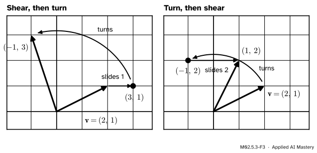
Compute \(\mat{R}\mat{S}\) and \(\mat{S}\mat{R}\) by the entry rule, and send \(\vect{v} = (2, 1)\) through both.
\(\mat{R}\mat{S}\). The rows of \(\mat{R}\) are \((0, -1)\) and \((1, 0)\). The columns of \(\mat{S}\) are \((1, 0)\) and \((1, 1)\).
The vector. By columns, \((\mat{R}\mat{S})\vect{v} = 2\,(0, 1) + 1\,(-1, 1) = (-1, 3)\) and \((\mat{S}\mat{R})\vect{v} = 2\,(1, 1) + 1\,(-1, 0) = (1, 2)\).
M02.5.3-F3
The vector \((2, 1)\) on its two journeys. Shear first, and it slides by its height, 1. Turn first, and by the time the shear acts it is at height 2, so it slides by 2.
Now check that brackets do not matter, with three maps: the shear, then \(\mat{T}\) of M02.4, then the quarter turn. That is the product \(\mat{R}\mat{T}\mat{S}\).
Group the left pair first. Lesson M02.5.1 found \(\mat{R}\mat{T} = \begin{bmatrix} 1 & -2 \\ 1 & 1 \end{bmatrix}\). Apply it to the columns of \(\mat{S}\): \((\mat{R}\mat{T})\,(1, 0) = (1, 1)\) and \((\mat{R}\mat{T})\,(1, 1) = (1, 1) + (-2, 1) = (-1, 2)\).
Group the right pair first.\(\mat{T}\mat{S}\) has columns \(\mat{T}\,(1, 0) = (1, -1)\) and \(\mat{T}\,(1, 1) = (1, -1) + (1, 2) = (2, 1)\). Apply \(\mat{R}\) to each: \(\mat{R}\,(1, -1) = (1, 1)\) and \(\mat{R}\,(2, 1) = 2\,(0, 1) + 1\,(-1, 0) = (-1, 2)\).
From scratch, with the three loops of M02.5.2 written compactly.
def matmul(A, B):"""A times B: entry (i, j) is row i of A times column j of B."""return [[sum(A[i][k] * B[k][j] for k inrange(len(B))) for j inrange(len(B[0]))]for i inrange(len(A))]def add(A, B):return [[a + b for a, b inzip(row_a, row_b)] for row_a, row_b inzip(A, B)]R = [[0, -1], [1, 0]] # quarter turnS = [[1, 1], [0, 1]] # shearT = [[1, 1], [-1, 2]] # the map of M02.4print("R S =", matmul(R, S), " S R =", matmul(S, R), " equal?", matmul(R, S) == matmul(S, R))print("(R T) S =", matmul(matmul(R, T), S), " R (T S) =", matmul(R, matmul(T, S)))print("T (S + R) =", matmul(T, add(S, R)), " T S + T R =", add(matmul(T, S), matmul(T, R)))
R S = [[0, -1], [1, 1]]   S R = [[1, -1], [1, 0]]   equal? False
(R T) S = [[1, -1], [1, 2]]   R (T S) = [[1, -1], [1, 2]]
T (S + R) = [[2, 1], [1, 2]]   T S + T R = [[2, 1], [1, 2]]
The two failures in the table, with the two projections:
P = [[1, 0], [0, 0]] # onto the horizontal axisQ = [[0, 0], [0, 1]] # onto the vertical axisZ = [[0, 0], [0, 0]] # the zero matrixprint("P Q =", matmul(P, Q), " although neither P nor Q is zero")print("P Q == P Z:", matmul(P, Q) == matmul(P, Z), " but Q == Z:", Q == Z)
P Q = [[0, 0], [0, 0]]   although neither P nor Q is zero
P Q == P Z: True   but Q == Z: False
Now NumPy, on random matrices. Rounding makes the two sides of a law differ in the last decimal places, so compare with np.allclose, not with ==.
import numpy as nprng = np.random.default_rng(0)commuting =0for _ inrange(1000): A, B, C = rng.normal(size=(3, 2, 2)) commuting += np.allclose(A @ B, B @ A)assert np.allclose((A @ B) @ C, A @ (B @ C)) # brackets can moveassert np.allclose(A @ (B + C), A @ B + A @ C) # distributes on the leftassert np.allclose((A + B) @ C, A @ C + B @ C) # and on the rightprint("random pairs that commute:", commuting, "of 1000")def rotation(degrees): a = np.deg2rad(degrees)return np.array([[np.cos(a), -np.sin(a)], [np.sin(a), np.cos(a)]])print("two rotations commute:", np.allclose(rotation(30) @ rotation(60), rotation(60) @ rotation(30)))n =1000print("multiplications for (AB)v:", n**3+ n**2, " for A(Bv):", 2* n**2, " ratio:", (n**3+ n**2) / (2* n**2))
random pairs that commute: 0 of 1000
two rotations commute: True
multiplications for (AB)v: 1001000000   for A(Bv): 2000000   ratio: 500.5
Explore
M02.5-X1
Composition explorer
Two maps, \(\mat{A}\) and \(\mat{B}\). Press Step to apply one and then the other, and watch the letter F arrive on the dashed outline: the place the single product matrix sends it. Press Swap the order to see where the other order leads. Every control is a button or a slider, so the keyboard works too.
Things to try:
Start with Shear and quarter turn and press Step twice. Where are \(\ihat\) and \(\jhat\) after each step? Compare with the columns of the product in the read-out.
Press Swap the order. The solid F jumps to where the dotted outline was. Step through again and find the moment at which the two orders part company.
Press Two rotations. The dotted outline has gone. What does the read-out say about \(\mat{A}\mat{B}\) and \(\mat{B}\mat{A}\)?
Press Two projections and step through. Where does the whole plane end up, and what is the product?
Press Same shear twice, then move the four sliders of \(\mat{B}\) one at a time. Which of them can you move without breaking \(\mat{A}\mat{B} = \mat{B}\mat{A}\)?
Pitfalls
M02.5.3-F4
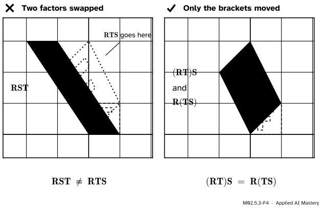
Wrong beside right. Swapping two neighbouring matrices gives a different map. Moving the brackets gives the same one.
“Brackets can move, so the matrices can move too.”
Associativity moves brackets and nothing else. \((\mat{R}\mat{T})\mat{S}\) and \(\mat{R}(\mat{T}\mat{S})\) are equal, both \(\begin{bmatrix} 1 & -1 \\ 1 & 2 \end{bmatrix}\). But swap two neighbours and you have a different product: \(\mat{R}\mat{S}\mat{T} = \begin{bmatrix} 1 & -2 \\ 0 & 3 \end{bmatrix}\). When you simplify a matrix expression, every matrix must keep its place in the line.
The middle terms are \(\mat{A}\mat{B} + \mat{B}\mat{A}\), and they combine into \(2\mat{A}\mat{B}\) only if the two matrices commute. For \(\mat{R}\) and \(\mat{S}\) the true square is \(\begin{bmatrix} 1 & 0 \\ 2 & 1 \end{bmatrix}\), and the school formula gives \(\begin{bmatrix} 0 & 0 \\ 2 & 2 \end{bmatrix}\).
“If \(\mat{A}\mat{B} = \mat{A}\mat{C}\), cancel \(\mat{A}\) to get \(\mat{B} = \mat{C}\).”
Dividing is not available. If \(\mat{A}\) squashes the plane, it sends many different vectors to the same place and can hide the difference between \(\mat{B}\) and \(\mat{C}\). With the projection \(\mat{P}\) we had \(\mat{P}\mat{Q} = \mat{P}\,\mat{0}\) although \(\mat{Q} \neq \mat{0}\). Cancelling is safe when \(\mat{A}\) can be undone, because the map that undoes \(\mat{A}\) can then be applied to both sides. Undoing a map is the subject of M02.7. The same warning covers “the product is zero, so one factor is zero”: the two projections show that it can fail.
Check yourself
Recall
1. Is \(\mat{A}\mat{B} = \mat{B}\mat{A}\) for all matrices? Give an example.
Show answer
No. For the shear \(\mat{S}\) and the quarter turn \(\mat{R}\), \(\mat{R}\mat{S} = \begin{bmatrix} 0 & -1 \\ 1 & 1 \end{bmatrix}\) and \(\mat{S}\mat{R} = \begin{bmatrix} 1 & -1 \\ 1 & 0 \end{bmatrix}\).
2. What does it mean for two matrices to commute? Name a pair that does.
Show answer
\(\mat{A}\mat{B} = \mat{B}\mat{A}\): the order makes no difference. Any two rotations of the plane commute, and so do any two stretches along the axes.
3. State the associative law, and say what it means for maps.
Show answer
\((\mat{A}\mat{B})\mat{C} = \mat{A}(\mat{B}\mat{C})\). Either way a vector meets \(\mat{C}\), then \(\mat{B}\), then \(\mat{A}\). The brackets only say which pair was merged first.
5. Give two non-zero matrices whose product is the zero matrix.
Show answer
The projections \(\mat{P} = \begin{bmatrix} 1 & 0 \\ 0 & 0 \end{bmatrix}\) and \(\mat{Q} = \begin{bmatrix} 0 & 0 \\ 0 & 1 \end{bmatrix}\): one drops the plane onto an axis, and the other drops that axis onto the origin.
Exercises
1.★ Let \(\mat{D} = \begin{bmatrix} 2 & 0 \\ 0 & 1 \end{bmatrix}\), a stretch sideways by a factor 2, and let \(\mat{S}\) be the shear. Compute \(\mat{D}\mat{S}\) and \(\mat{S}\mat{D}\), and explain the difference in words.
They differ in the top right entry. Shear first, and the one-unit slide of \(\jhat\) is then stretched to two units. Stretch first, and \(\jhat\), which lies on the vertical axis, is not stretched at all, so it slides by just one unit.
2.★★ (a) Show that any two shears along the horizontal axis commute, by computing \(\begin{bmatrix} 1 & k \\ 0 & 1 \end{bmatrix}\begin{bmatrix} 1 & l \\ 0 & 1 \end{bmatrix}\) in both orders. (b) Show that any two matrices of the form \(\begin{bmatrix} a & 0 \\ 0 & d \end{bmatrix}\) commute.
Show solution
(a) By the entry rule,
\[
\begin{aligned}
&\begin{bmatrix} 1 & k \\ 0 & 1 \end{bmatrix}\begin{bmatrix} 1 & l \\ 0 & 1 \end{bmatrix} \\[0.4em]
&\quad= \begin{bmatrix} 1 \cdot 1 + k \cdot 0 & 1 \cdot l + k \cdot 1 \\ 0 \cdot 1 + 1 \cdot 0 & 0 \cdot l + 1 \cdot 1 \end{bmatrix} \\[0.4em]
&\quad= \begin{bmatrix} 1 & l + k \\ 0 & 1 \end{bmatrix}.
\end{aligned}
\]
Swapping \(k\) and \(l\) gives \(\begin{bmatrix} 1 & k + l \\ 0 & 1 \end{bmatrix}\), the same matrix. Sliding by \(l\) times the height and then by \(k\) times the height is one slide by \(k + l\) times the height, in either order.
(b) \(\begin{bmatrix} a & 0 \\ 0 & d \end{bmatrix}\begin{bmatrix} e & 0 \\ 0 & h \end{bmatrix}
= \begin{bmatrix} ae & 0 \\ 0 & dh \end{bmatrix}\), and the other order gives \(\begin{bmatrix} ea & 0 \\ 0 & hd \end{bmatrix}\). These are equal because numbers commute.
3.★★★ Suppose a \(2 \times 2\) matrix \(\mat{A}\) commutes with every\(2 \times 2\) matrix. Show that \(\mat{A}\) is a multiple of the identity matrix, \(\begin{bmatrix} a & 0 \\ 0 & a \end{bmatrix}\), and that every such multiple does commute with everything.
Show solution
Write \(\mat{A} = \begin{bmatrix} a & b \\ c & d \end{bmatrix}\). It must commute with the projection \(\mat{P} = \begin{bmatrix} 1 & 0 \\ 0 & 0 \end{bmatrix}\). By the column rule,
\[
\begin{aligned}
\mat{A}\mat{P} &= \begin{bmatrix} a & 0 \\ c & 0 \end{bmatrix}, \\[0.5em]
\mat{P}\mat{A} &= \begin{bmatrix} a & b \\ 0 & 0 \end{bmatrix}.
\end{aligned}
\]
These are equal only if \(b = 0\) and \(c = 0\). So \(\mat{A} = \begin{bmatrix} a & 0 \\ 0 & d \end{bmatrix}\). It must also commute with the shear \(\mat{S}\):
\[
\begin{aligned}
\mat{A}\mat{S} &= \begin{bmatrix} a & a \\ 0 & d \end{bmatrix}, \\[0.5em]
\mat{S}\mat{A} &= \begin{bmatrix} a & d \\ 0 & d \end{bmatrix}.
\end{aligned}
\]
These are equal only if \(a = d\). So \(\mat{A} = a\begin{bmatrix} 1 & 0 \\ 0 & 1 \end{bmatrix}\).
In the other direction, let \(\mat{I}\) be the identity matrix, the map that moves nothing. For any \(\mat{B}\) and any \(\vect{v}\), both \((a\mat{I})\mat{B}\) and \(\mat{B}(a\mat{I})\) send \(\vect{v}\) to \(a\,\mat{B}\vect{v}\): scaling by \(a\) before or after \(\mat{B}\) is the same, by homogeneity. So \(a\mat{I}\) commutes with every matrix.
Summary card
The order of a product matters. Its brackets do not.
M02.5.3-F1
Two orders, two results.
Not commutative. Usually \(\mat{A}\mat{B} \neq \mat{B}\mat{A}\). When they are equal, the two matrices commute.
Associative.\((\mat{A}\mat{B})\mat{C} = \mat{A}(\mat{B}\mat{C})\): first \(\mat{C}\), then \(\mat{B}\), then \(\mat{A}\).
No cancelling.\(\mat{A}\mat{B} = \mat{0}\) does not force a zero factor, and \(\mat{A}\mat{B} = \mat{A}\mat{C}\) does not force \(\mat{B} = \mat{C}\).
Sources and next steps
Sources. Each was opened and checked against this lesson on 12 November 2026.
Sheldon Axler, Linear Algebra Done Right, 4th edition (open access). Section 3A, result 3.8, lists the algebraic properties of products of linear maps: associativity and the two distributive properties. The text after it states that multiplication of linear maps is not commutative. Section 3C repeats all three statements for matrices, and its Exercise 12 asks for a clean proof of associativity, in the spirit of a remark of Emil Artin that it quotes: proofs about matrices get shorter “if one throws the matrices out”.
Marc Deisenroth, Aldo Faisal and Cheng Soon Ong, Mathematics for Machine Learning, Cambridge University Press, 2020 (free PDF). Section 2.2.1 states associativity (2.18) and distributivity (2.19a, 2.19b), and that matrix multiplication is not commutative. Section 5.6.2 is the source of the frontier note: forward and reverse mode differ in the order of multiplication, by associativity (equations 5.120 and 5.121), and reverse mode is backpropagation.
Grant Sanderson, Matrix multiplication as composition, 3Blue1Brown, Linear Algebra, chapter 4. Shows that order matters with a shear and a \(90°\) rotation, and argues for associativity as this lesson does: both bracketings apply the same three transformations in the same order.
Next.M02.5.4 Shapes, identity and powers asks which products exist at all, what multiplying a matrix by itself means, and what all this says about a stack of neural-network layers.