\( \newcommand{\vect}[1]{\mathbf{#1}} \newcommand{\mat}[1]{\mathbf{#1}} \newcommand{\R}{\mathbb{R}} \newcommand{\E}{\mathbb{E}} \newcommand{\Prob}{\mathbb{P}} \newcommand{\T}{^{\top}} \newcommand{\norm}[1]{\lVert #1 \rVert} \newcommand{\abs}[1]{\lvert #1 \rvert} \newcommand{\ihat}{\mkern1mu\hat{\boldsymbol{\imath}}\mkern2mu} \newcommand{\jhat}{\mkern1mu\hat{\boldsymbol{\jmath}}\mkern2mu} \newcommand{\pd}[2]{\frac{\partial #1}{\partial #2}} \newcommand{\argmax}{\operatorname*{arg\,max}} \newcommand{\argmin}{\operatorname*{arg\,min}} \newcommand{\cdata}[1]{\class{c-data}{#1}} \newcommand{\cmodel}[1]{\class{c-model}{#1}} \newcommand{\ctruth}[1]{\class{c-truth}{#1}} \newcommand{\cgrad}[1]{\class{c-grad}{#1}} \newcommand{\closs}[1]{\class{c-loss}{#1}} \newcommand{\cparam}[1]{\class{c-param}{#1}} \newcommand{\csecond}[1]{\class{c-second}{#1}} \renewcommand{\,}{\mkern3mu} \)

Linear combinations

Scale some vectors and add the results: that single move is a linear combination, and the rest of linear algebra is built from it. Learn to compute one, to draw it tip to tail, and to find the weights that reach a target, by picture and by solving two equations.

M02.2.1L1 Core25 minIn review

Before this lesson

M02.1 Vectors as arrows and as data

After this lesson you can

Compute a linear combination of two or more vectors from its weights, in coordinates and as a tip-to-tail picture.
Read the weights of a point off the slanted grid that two vectors draw.
Find the weights that reach a target in the plane by solving two equations, and check the answer.
Recognise the weighted sums of machine learning, such as the predictions of a linear model, as linear combinations.

In review. The maths and code on this page are checked by automated tests on every change, but an independent reader has not signed it off yet. Spot a mistake or a confusing step? Tell us.

The question

A model that prices houses multiplies each feature by a weight and adds the results. A neural network does the same thing many times over in every layer. Both are one move: scale some vectors, then add them. What can that one move reach, and if you know where you want to land, how do you find the weights that take you there?

Intuition

Module M02.1 gave vectors two operations. You can scale a vector by a number, and you can add two vectors tip to tail. A linear combination does both at once: scale each vector by its own number, then add the results. The numbers are called weights.

Think of a recipe. The vectors are the ingredients and the weights say how much of each to use: “2 of \(\vect{u}\) and 1 of \(\vect{v}\)”.

M02.2.1-F1

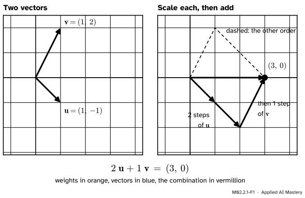
A linear combination of \(\vect{u} = (1, -1)\) and \(\vect{v} = (1, 2)\) with weights 2 and 1. Walk two steps of \(\vect{u}\), then one step of \(\vect{v}\), and you arrive at \((3, 0)\). These two vectors are the running pair of this module.

Read the right panel as a walk. Each weight says how many steps to take along its vector. The combination is the place where the walk ends.

Build it up

Step 1. One vector, one weight. Start with a single vector \(\vect{u}\) and a weight \(c\). The result \({c\,\vect{u}}\) is a stretched copy of \(\vect{u}\). With \(c = 2\) it is twice as long. With \(c = -1\) it points the opposite way. With \(c = 0\) it is the zero vector. As \(c\) changes, the tip of \({c\,\vect{u}}\) slides along one straight line through the origin.

Step 2. Two vectors, two weights. Now take \({a\,\vect{u}} + {b\,\vect{v}}\). Walk \(a\) steps of \(\vect{u}\), then \(b\) steps of \(\vect{v}\). For the figure, \({2\,\vect{u}} = (2, -2)\) and \({1\,\vect{v}} = (1, 2)\), and their sum is \((2 + 1,\; -2 + 2) = (3, 0)\).

Step 3. The order does not matter. Take the step of \(\vect{v}\) first and the two steps of \(\vect{u}\) second: \((1, 2) + (2, -2) = (3, 0)\), the same point. That is the dashed path in the figure. Adding vectors in either order gives the same result (lesson M02.1.3), so the two routes are the two halves of one parallelogram.

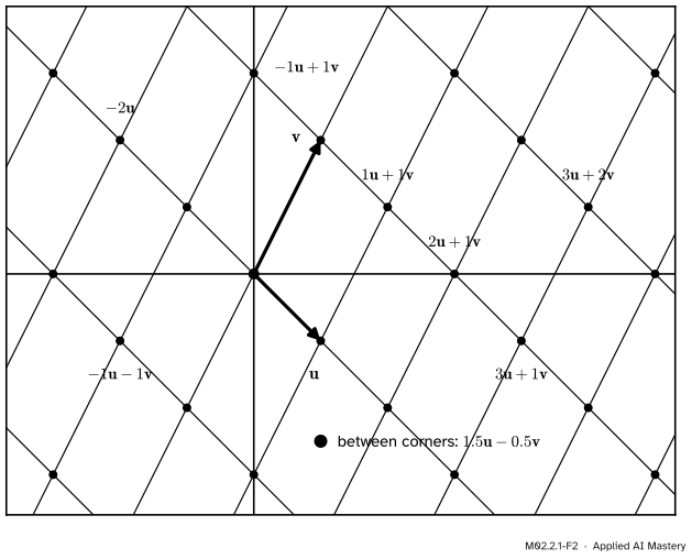
Step 4. Whole-number weights draw a slanted grid. Mark every point you can reach with whole-number weights. The marks form a grid, but a slanted one: its lines run along \(\vect{u}\) and along \(\vect{v}\) instead of along the axes.

M02.2.1-F2

Every corner of the slanted grid is a combination with whole-number weights, so every corner has an address: its pair of weights. Points inside a cell need weights that are not whole numbers.

Weights do not have to be whole numbers. The vermillion point is \({1.5\,\vect{u}} - {0.5\,\vect{v}} = (1.5 - 0.5,\; -1.5 - 1) = (1, -2.5)\). It sits inside a cell.

Step 5. Turn the question round. So far the weights were given and the point was the answer. The more useful question runs the other way: here is a target, which weights reach it? On the picture you can count steps along the slanted grid. The next section turns that counting into two equations.

The formal statement

Definition: linear combination

Let \(\vect{v}_1, \dots, \vect{v}_k\) be vectors in \(\R^n\) and let \(c_1, \dots, c_k\) be real numbers. The vector

\[ c_1\,\vect{v}_1 + c_2\,\vect{v}_2 + \cdots + c_k\,\vect{v}_k \]

is a linear combination of \(\vect{v}_1, \dots, \vect{v}_k\). The numbers \(c_1, \dots, c_k\) are its weights (also called coefficients).

Any number of vectors may be combined, in any dimension, and each weight may be any real number: positive, negative, a fraction, or zero.

In coordinates. For two vectors in the plane, scale entry by entry and add entry by entry (lesson M02.1.3):

\[ \begin{aligned} \cparam{a}\,\cdata{\vect{u}} + \cparam{b}\,\cdata{\vect{v}} &= \cparam{a}\begin{bmatrix} u_1 \\ u_2 \end{bmatrix} + \cparam{b}\begin{bmatrix} v_1 \\ v_2 \end{bmatrix} \\[4pt] &= \begin{bmatrix} a u_1 \\ a u_2 \end{bmatrix} + \begin{bmatrix} b v_1 \\ b v_2 \end{bmatrix} \\[4pt] &= \cmodel{\begin{bmatrix} a u_1 + b v_1 \\ a u_2 + b v_2 \end{bmatrix}} . \end{aligned} \]

The weights multiply the vectors, and the combination comes out.

Finding the weights. To reach a target \(\vect{t} = (t_1, t_2)\) we need \({a\,\vect{u}} + {b\,\vect{v}} = \vect{t}\). Two vectors are equal exactly when their entries match, so this is two ordinary equations in the two unknowns \(a\) and \(b\):

\[ \begin{aligned} a u_1 + b v_1 &= t_1 && \text{(first entries)} \\ a u_2 + b v_2 &= t_2 && \text{(second entries)} \end{aligned} \]

To find \(a\), remove \(b\). Multiply the first equation by \(v_2\) and the second by \(v_1\), so that both contain the same term \(b v_1 v_2\), then subtract the second from the first:

\[ \begin{aligned} a u_1 v_2 + b v_1 v_2 &= t_1 v_2 \\ a u_2 v_1 + b v_1 v_2 &= t_2 v_1 \\[2pt] a\,(u_1 v_2 - u_2 v_1) &= t_1 v_2 - t_2 v_1 . \end{aligned} \]

To find \(b\), remove \(a\) the same way. Multiply the first equation by \(u_2\) and the second by \(u_1\), then subtract the first from the second:

\[ \begin{aligned} a u_1 u_2 + b v_1 u_2 &= t_1 u_2 \\ a u_1 u_2 + b v_2 u_1 &= t_2 u_1 \\[2pt] b\,(u_1 v_2 - u_2 v_1) &= u_1 t_2 - u_2 t_1 . \end{aligned} \]

The same number multiplies both unknowns. Call it \(D = u_1 v_2 - u_2 v_1\), so that the two results read \(aD = t_1 v_2 - t_2 v_1\) and \(bD = u_1 t_2 - u_2 t_1\). If \(D \neq 0\) we can divide by it:

\[ \begin{gathered} a = \frac{t_1 v_2 - t_2 v_1}{D}, \\[4pt] b = \frac{u_1 t_2 - u_2 t_1}{D} . \end{gathered} \]

This shows that if some weights reach the target, they must be these two. It remains to check that these two really do reach it. Take the first entry, \(a u_1 + b v_1\), and multiply it by \(D\):

\[ \begin{aligned} &(aD)\,u_1 + (bD)\,v_1 \\ &= (t_1 v_2 - t_2 v_1) u_1 \\ &\quad + (u_1 t_2 - u_2 t_1) v_1 \\ &= t_1 u_1 v_2 - t_2 u_1 v_1 \\ &\quad + t_2 u_1 v_1 - t_1 u_2 v_1 \\ &= t_1\,(u_1 v_2 - u_2 v_1) \\ &= t_1\,D . \end{aligned} \]

The two middle terms, \(-t_2 u_1 v_1\) and \(+t_2 u_1 v_1\), cancel. Dividing by \(D\) gives \(a u_1 + b v_1 = t_1\). The second entry works the same way:

\[ \begin{aligned} &(aD)\,u_2 + (bD)\,v_2 \\ &= (t_1 v_2 - t_2 v_1) u_2 \\ &\quad + (u_1 t_2 - u_2 t_1) v_2 \\ &= t_1 u_2 v_2 - t_2 u_2 v_1 \\ &\quad + t_2 u_1 v_2 - t_1 u_2 v_2 \\ &= t_2\,(u_1 v_2 - u_2 v_1) \\ &= t_2\,D . \end{aligned} \]

Here the first and last terms cancel. Dividing by \(D\) gives \(a u_2 + b v_2 = t_2\), so both entries match the target.

Result: one target, one pair of weights

Let \(\vect{u}\) and \(\vect{v}\) be vectors in the plane with \(D = u_1 v_2 - u_2 v_1 \neq 0\). Then every target \(\vect{t}\) is reached by exactly one pair of weights. That is, \(\vect{t} = {a\,\vect{u}} + {b\,\vect{v}}\) holds for

\[ \begin{gathered} a = \frac{t_1 v_2 - t_2 v_1}{D}, \\[4pt] b = \frac{u_1 t_2 - u_2 t_1}{D} \end{gathered} \]

and for no other weights.

When \(D = 0\) the division is not allowed and the result says nothing. The next lesson shows that this happens exactly when \(\vect{u}\) and \(\vect{v}\) lie along one line. The number \(D\) returns in module M02.8 as the determinant.

Go deeper: weights that add up to one: blends and averages

A special kind of combination appears all over machine learning: two weights that add up to one. Write the weights as \(a\) and \(1 - a\). Then

\[ \begin{aligned} &a\,\vect{u} + (1 - a)\,\vect{v} \\ &\;= \vect{v} + a\,\vect{u} - a\,\vect{v} \\ &\;= \vect{v} + a\,(\vect{u} - \vect{v}) . \end{aligned} \]

The right-hand side starts at the tip of \(\vect{v}\) and moves a fraction \(a\) of the way along \(\vect{u} - \vect{v}\), the arrow from the tip of \(\vect{v}\) to the tip of \(\vect{u}\) (lesson M02.1.3). So the combination lies on the line through the two tips. With \(a = 0\) it is \(\vect{v}\), with \(a = 1\) it is \(\vect{u}\), and with \(a = \tfrac12\) it is the midpoint. For \(0 \le a \le 1\) it stays on the segment between the tips, and it is then called a weighted average or a blend.

The Adam optimiser (Kingma and Ba, 2014) trains a model from a gradient \(\vect{g}\), a noisy vector that says how to change the weights, and it keeps a running average \(\vect{m}\) of that vector in exactly this way. With its default setting the update is

\[ \vect{m} \leftarrow 0.9\,\vect{m} + 0.1\,\vect{g} , \]

a blend that keeps nine tenths of the old value and takes one tenth of the new one.

Worked example

Reach the target \((5, 1)\) with \(\vect{u} = (1, -1)\) and \(\vect{v} = (1, 2)\).

M02.2.1-F3

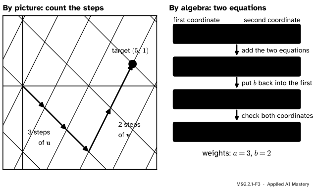
The same answer found twice. On the left, count steps along the slanted grid. On the right, write one equation for each coordinate and solve.

By picture. Follow the grid lines from the origin. Three steps of \(\vect{u}\) and then two steps of \(\vect{v}\) end on the target, so the weights are \(a = 3\) and \(b = 2\).

By algebra. The combination is \({a\,(1, -1)} + {b\,(1, 2)} = (a + b,\; -a + 2b)\). Match each entry to the target:

\[ \begin{aligned} a + b &= 5 \\ -a + 2b &= 1 \end{aligned} \]

Add the two equations. The terms \(a\) and \(-a\) cancel and leave \(3b = 6\), so \(b = 2\). Put that back into the first equation: \(a = 5 - 2 = 3\).

Check. \({3\,(1, -1)} + {2\,(1, 2)} = (3 + 2,\; -3 + 4) = (5, 1)\). Both entries match.

By the formula. Here \(D = {1 \cdot 2} - {(-1) \cdot 1} = 3\), so

\[ \begin{aligned} a &= \frac{5 \cdot 2 - 1 \cdot 1}{3} = \frac{9}{3} = 3, \\[4pt] b &= \frac{1 \cdot 1 - (-1) \cdot 5}{3} = \frac{6}{3} = 2 . \end{aligned} \]

A target with awkward weights. For \(\vect{t} = (-1,\, 2.5)\) the same formula gives

\[ \begin{aligned} a &= \frac{(-1) \cdot 2 - 2.5 \cdot 1}{3} = \frac{-4.5}{3} \\[2pt] &= -1.5, \\[4pt] b &= \frac{1 \cdot 2.5 - (-1)(-1)}{3} = \frac{1.5}{3} \\[2pt] &= 0.5 . \end{aligned} \]

Check: \({-1.5\,(1, -1)} + {0.5\,(1, 2)} = (-1.5 + 0.5,\; 1.5 + 1) = (-1,\, 2.5)\). A negative weight means walking backwards along that vector, and a fraction means part of a step.

More entries: a linear model. Three houses have sizes \(\vect{s} = (50, 80, 120)\) in square metres and \(\vect{r} = (1, 2, 4)\) bedrooms. A linear model with weight 3 on size and weight 20 on bedrooms predicts the prices (in thousands)

\[ \begin{aligned} &3\,\vect{s} + 20\,\vect{r} \\ &\;= 3\,(50, 80, 120) + 20\,(1, 2, 4) \\ &\;= (150, 240, 360) + (20, 40, 80) \\ &\;= (170,\, 280,\, 440) . \end{aligned} \]

The model’s weights are the weights of a linear combination, and the vectors being combined are the columns of features. Nothing changed except the number of entries.

Frontier note: arithmetic on word vectors

A word embedding stores each word as a vector (lesson M02.1.4). Mikolov and colleagues reported in 2013 that simple combinations of such vectors carry meaning: the combination \(\vect{v}_{\text{king}} - \vect{v}_{\text{man}} + \vect{v}_{\text{woman}}\), with weights \(1\), \(-1\) and \(1\), gives a vector whose nearest word vector is that of queen. The paper set out to build models that preserve such linear regularities among words.

Code

First from scratch, with vectors as plain tuples. A linear combination is a loop that scales and adds.

def scale(c, v):
    return tuple(c * x for x in v)

def add(u, v):
    return tuple(x + y for x, y in zip(u, v))

def combine(weights, vectors):
    """Scale each vector by its weight, then add the results."""
    total = (0,) * len(vectors[0])
    for c, v in zip(weights, vectors):
        total = add(total, scale(c, v))
    return total

u, v = (1, -1), (1, 2)
print("2u + 1v =", combine([2, 1], [u, v]))
print("1v + 2u =", combine([1, 2], [v, u]))
print("3u + 2v =", combine([3, 2], [u, v]))
print("1.5u - 0.5v =", combine([1.5, -0.5], [u, v]))

2u + 1v = (3, 0)
1v + 2u = (3, 0)
3u + 2v = (5, 1)
1.5u - 0.5v = (1.0, -2.5)

Now the reverse question. This function is the formula from the formal section, line for line.

def find_weights(u, v, t):
    """The weights a, b with a*u + b*v = t, for vectors in the plane."""
    D = u[0] * v[1] - u[1] * v[0]
    if D == 0:
        raise ValueError("u and v lie along one line: the formula does not apply")
    a = (t[0] * v[1] - t[1] * v[0]) / D
    b = (u[0] * t[1] - u[1] * t[0]) / D
    return a, b

print("target (5, 1):   ", find_weights(u, v, (5, 1)))
print("target (-1, 2.5):", find_weights(u, v, (-1, 2.5)))

target (5, 1):    (3.0, 2.0)
target (-1, 2.5): (-1.5, 0.5)

With NumPy a linear combination is one line, because arrays scale and add entry by entry. To find weights, put the vectors side by side as columns and call np.linalg.solve, which solves the same two equations.

import numpy as np

u, v = np.array([1.0, -1.0]), np.array([1.0, 2.0])
print("3u + 2v =", 3 * u + 2 * v)

columns = np.column_stack([u, v])        # u and v side by side
print("weights for (5, 1):", np.linalg.solve(columns, [5, 1]))

size, bedrooms = np.array([50, 80, 120]), np.array([1, 2, 4])
print("predicted prices:", 3 * size + 20 * bedrooms)

3u + 2v = [5. 1.]
weights for (5, 1): [3. 2.]
predicted prices: [170 280 440]

Explore

This module’s interactive, the span explorer, lives in the next lesson. It has a slider for each weight and a target to reach, so it is a good place to practise this lesson: set a target, guess the weights, then let it show you the answer.

Pitfalls

M02.2.1-F4

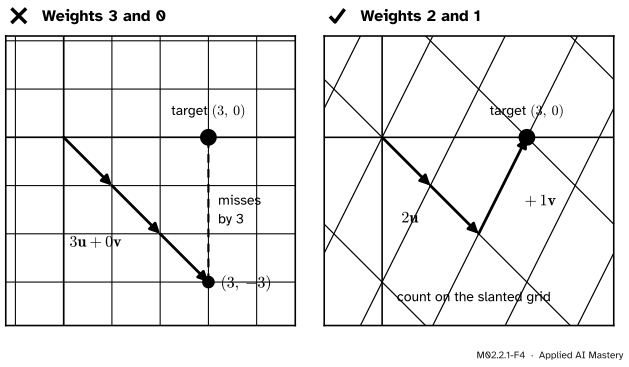
Wrong beside right. The target’s ordinary coordinates, 3 and 0, are not the weights. The weights are counted along \(\vect{u}\) and \(\vect{v}\).

“The target is \((3, 0)\), so the weights are 3 and 0.”

The entries of the target say how far to go along the axes. The weights say how far to go along \(\vect{u}\) and \(\vect{v}\). These are different questions: \({3\,\vect{u}} + {0\,\vect{v}} = (3, -3)\), which misses, while \({2\,\vect{u}} + {1\,\vect{v}} = (3, 0)\). Lesson M02.2.4 gives the weights a name: the coordinates of the point in the basis \(\vect{u}, \vect{v}\).

“Weights are positive whole numbers, like amounts in a recipe.”

Any real number is allowed. A negative weight walks backwards, a fraction takes part of a step, and a zero leaves the vector out. The weights that a model learns are typically fractions, positive and negative alike.

“Adding a constant, or multiplying two vectors together, is still a linear combination.”

Only two moves are allowed: scale, and add. The rule \({a\,\vect{u}} + {b\,\vect{v}} + (1, 1)\) has a third move, a fixed shift that no weight controls. With both weights zero it gives \((1, 1)\), where a linear combination of \(\vect{u}\) and \(\vect{v}\) gives \(\vect{0}\). Multiplying the entries of \(\vect{u}\) by those of \(\vect{v}\) is not one of the two moves either. The shift is the difference between the linear part \(\mat{W}\vect{x}\) of a network layer and its bias \(\vect{b}\), which lesson M02.4.1 takes up.

Check yourself

Recall

1. What is a linear combination of \(\vect{u}\) and \(\vect{v}\)?

Show answer

A vector of the form \({a\,\vect{u}} + {b\,\vect{v}}\), where the numbers \(a\) and \(b\) are called the weights: scale each vector, then add.

2. Compute \({2\,(1, -1)} + {1\,(1, 2)}\).

Show answer

\((2 + 1,\; -2 + 2) = (3, 0)\).

3. What shape do the points with whole-number weights make?

Show answer

The corners of a slanted grid, whose lines run along \(\vect{u}\) and along \(\vect{v}\).

4. Which two equations say that \({a\,\vect{u}} + {b\,\vect{v}} = \vect{t}\) in the plane?

Show answer

One for each entry: \(a u_1 + b v_1 = t_1\) and \(a u_2 + b v_2 = t_2\).

5. Which number must not be zero for the formula to give the weights?

Show answer

\(D = u_1 v_2 - u_2 v_1\). When \(D \neq 0\), every target has exactly one pair of weights.

Exercises

1. ★ Let \(\vect{u} = (2, 1)\) and \(\vect{v} = (-1, 3)\). Compute \({3\,\vect{u}} - {2\,\vect{v}}\) and \({\tfrac12\,\vect{u}} + \vect{v}\).

Show solution

\({3\,(2, 1)} - {2\,(-1, 3)} = (6 + 2,\; 3 - 6) = (8, -3)\).

\({\tfrac12\,(2, 1)} + (-1, 3) = (1 - 1,\; 0.5 + 3) = (0,\, 3.5)\).

2. ★★ With the same \(\vect{u} = (2, 1)\) and \(\vect{v} = (-1, 3)\), find the weights that reach the target \((4, 9)\). Check your answer.

Show solution

The equations are \(2a - b = 4\) and \(a + 3b = 9\). From the first, \(b = 2a - 4\). Substitute into the second: \(a + 3(2a - 4) = 9\), so \(7a = 21\) and \(a = 3\). Then \(b = {2 \cdot 3} - 4 = 2\).

Check: \({3\,(2, 1)} + {2\,(-1, 3)} = (6 - 2,\; 3 + 6) = (4, 9)\).

The formula agrees: \(D = {2 \cdot 3} - {1 \cdot (-1)} = 7\), \(a = ({4 \cdot 3} - {9 \cdot (-1)})/7 = 21/7 = 3\) and \(b = ({2 \cdot 9} - {1 \cdot 4})/7 = 14/7 = 2\).

3. ★★★ Let \(\vect{u} = (1, 2)\) and \(\vect{v} = (2, 4)\). Show that no weights reach the target \((3, 5)\), and that more than one pair of weights reaches \((3, 6)\). What is \(D\)?

Show solution

For \((3, 5)\) the equations are \(a + 2b = 3\) and \(2a + 4b = 5\). Twice the first equation says \(2a + 4b = 6\), which contradicts the second. No weights exist.

For \((3, 6)\) the equations are \(a + 2b = 3\) and \(2a + 4b = 6\). The second is twice the first, so there is really only one condition, \(a = 3 - 2b\), and every choice of \(b\) works: \((a, b) = (3, 0)\), \((1, 1)\) and \((-1, 2)\) all reach it. For example \({1\,(1, 2)} + {1\,(2, 4)} = (3, 6)\).

Here \(D = {1 \cdot 4} - {2 \cdot 2} = 0\), so the result of this lesson does not apply. The reason is that \(\vect{v} = {2\,\vect{u}}\): both vectors lie along one line. The next two lessons are about exactly this situation.

Summary card

Scale each vector by its weight, then add.

The anchor figure again: on the left the vectors u equals (1, minus 1) and v equals (1, 2); on the right a walk of two steps of u and one step of v that ends at (3, 0), with the equation 2u plus 1v equals (3, 0) underneath. — M02.2.1-F1
Two steps of one, one of the other.

Linear combination. \(c_1\vect{v}_1 + \cdots + c_k\vect{v}_k\), with weights \(c_1, \dots, c_k\).
In the plane. \({a\,\vect{u}} + {b\,\vect{v}} = (a u_1 + b v_1,\; a u_2 + b v_2)\).
Reaching a target. Solve \(a u_1 + b v_1 = t_1\) and \(a u_2 + b v_2 = t_2\).
The weights. If \(D = u_1 v_2 - u_2 v_1 \neq 0\), then \(a = (t_1 v_2 - t_2 v_1)/D\) and \(b = (u_1 t_2 - u_2 t_1)/D\), and no other weights work.

Sources and next steps

Sources. Each was opened and checked against this lesson on 12 November 2026.

Sheldon Axler, Linear Algebra Done Right, 4th edition (open access). Section 2A, definition 2.2: a linear combination of a list of vectors is a sum of scalar multiples of them. Example 2.3 tests whether a vector is a combination by solving equations.
Grant Sanderson, Linear combinations, span, and basis vectors, 3Blue1Brown, Linear Algebra, chapter 2. The source of the picture: scaling two vectors and adding them is called a linear combination of those two vectors.
Marc Deisenroth, Aldo Faisal and Cheng Soon Ong, Mathematics for Machine Learning (free PDF). Section 2.5, definition 2.11 (linear combination).
Tomas Mikolov, Kai Chen, Greg Corrado and Jeffrey Dean (2013), Efficient Estimation of Word Representations in Vector Space. Section 1.1 reports the king, man, woman, queen example quoted in the frontier note.
Diederik Kingma and Jimmy Ba (2014), Adam: A Method for Stochastic Optimization. Algorithm 1 keeps a moving average of the gradient: each step takes \(\beta_1\) times the old average plus \(1 - \beta_1\) times the new gradient, with the default \(\beta_1 = 0.9\). That is the blend in the note on weights that add up to one.
NumPy reference, numpy.linalg.solve: it solves a square, full-rank linear system and raises LinAlgError when the matrix is singular.

Next. M02.2.2 Span: everything you can reach fixes the vectors, lets the weights run over all numbers, and asks what set of points comes out.

This lesson unlocks

M02.2.2 Span: everything you can reach

Your progress is saved in this browser only. No account, no tracking.