A house, a picture and a word can each be written as a list of numbers, which makes each one a point in space. Learn to measure the distance between data points, see why the unit of a feature changes the answer, and take a first look at high dimensions.
Turn a described object, such as a house or a small picture, into a feature vector and state its dimension.
Compute the distance between two data points as the length of their difference.
Show with numbers that changing the unit of one feature can change which data point is nearest, and rescale the features to prevent it.
Describe one way in which distances in high dimensions behave differently from distances in the plane.
In review. The maths and code on this page are checked by automated tests on every change, but an independent reader has not signed it off yet. Spot a mistake or a confusing step? Tell us.
The question
A property website says two houses are “similar”. A photo app groups pictures that “look alike”. A translation app treats king and queen as related words. A computer has no feeling for likeness. It has arithmetic. How do you turn houses, pictures and words into numbers in such a way that “similar” becomes “close together”?
From the last lesson
1. For \(\vect{u} = (1, 2)\) and \(\vect{v} = (3, 1)\), what is \(\vect{v} - \vect{u}\), and where does its arrow run when both vectors are drawn from the origin?
Show answer
\(\vect{v} - \vect{u} = (3 - 1,\; 1 - 2) = (2, -1)\). It runs from the tip of \(\vect{u}\) to the tip of \(\vect{v}\).
2. What does scaling a vector by the number \(c\) do to its length?
Show answer
It multiplies the length by \(\abs{c}\): \(\norm{c\vect{v}} = \abs{c}\,\norm{\vect{v}}\).
Intuition
Measure a few things about an object and write the measurements down in a fixed order. Each measurement is called a feature, and the list is the object’s feature vector. Do this for every object in a collection and each one becomes a vector with the same number of coordinates, which is to say a point in the same space.
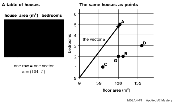
M02.1.4-F1
A table of data is a stack of vectors, one for each row. Drawn in the plane of its two features, each house is a point: the tip of its vector. From here on we draw only the dots.
Once objects are points, “how alike are these two?” becomes a question about geometry: how far apart are their points? That one move, from likeness to distance, is behind recommending songs, grouping customers and recognising handwriting.
Build it up
Step 1. A house. Describe a house by its floor area in square metres and its number of bedrooms. House A, with 104 square metres and 5 bedrooms, is the vector \(\vect{a} = (104, 5)\) in \(\R^2\). The order is fixed once and kept: area first, bedrooms second.
Step 2. More features. Add the number of bathrooms and the age in years and each house is a vector in \(\R^4\). Real tables have hundreds of columns. The picture is lost, but the arithmetic of lessons M02.1.2 and M02.1.3 carries on unchanged.
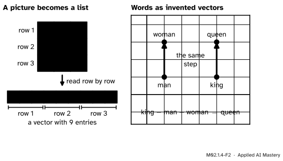
Step 3. A picture. A grey picture is a grid of pixels, each holding one number: here, the amount of ink from 0 to 1. Read the grid row by row and you have a list. A 3 by 3 picture is a vector in \(\R^9\), and a 28 by 28 picture is a vector in \(\R^{784}\).
Step 4. A word. Nobody can measure the “features” of a word with a ruler. A model learns them from a great deal of text, giving every word a vector of a few hundred numbers called a word embedding. Words used in similar ways end up with nearby vectors. More surprisingly, differences between vectors carry meaning: in a well-known experiment, the vector for king, minus the vector for man, plus the vector for woman, was closest to the vector for queen.
M02.1.4-F2
Left: a tiny picture of the letter T, flattened row by row into a vector in \(\R^9\). Right: four invented two-number word vectors, chosen so that the step from man to woman is exactly the step from king to queen. Real embeddings have hundreds of coordinates and the match is only approximate.
In the toy picture, \(\text{king} - \text{man} + \text{woman} = (4 - 1 + 1,\; 1 - 1 + 3) = (4, 3)\), which is the vector for queen. It works because \(\text{woman} - \text{man}\) and \(\text{queen} - \text{king}\) are the same vector, \((0, 2)\).
Step 5. Distance. Lesson M02.1.3 showed that \(\vect{a} - \vect{b}\) is the arrow that joins the tips of \(\vect{b}\) and \(\vect{a}\). The length of that arrow is how far apart the two points are. So the distance between two data points is the length of their difference.
Step 6. Units. The distance formula treats every coordinate alike: a difference of 1 square metre counts exactly as much as a difference of 1 bedroom. Whether that is sensible depends on the units, and the worked example shows that it can decide the answer.
The formal statement
NoteDefinition: distance
The distance between two vectors \(\vect{a}\) and \(\vect{b}\) in \(\R^n\) is the length of their difference:
In the plane and in space this is the ordinary straight-line distance between the two points, because \(\vect{a} - \vect{b}\) is the arrow from one to the other and lesson M02.1.2 showed that the formula gives the length of an arrow. For \(n \ge 4\) it is the definition of distance. Four facts follow from the formula.
Fact 1: the order does not matter.\(\operatorname{dist}(\vect{a}, \vect{b}) = \operatorname{dist}(\vect{b}, \vect{a})\), because \(b_i - a_i = -(a_i - b_i)\) and squaring removes the sign: \((b_i - a_i)^2 = (a_i - b_i)^2\) in every term.
Fact 2: only identical points are at distance zero. Each term \((a_i - b_i)^2\) is zero or more, so the distance is zero or more. A sum of such terms is zero only when every term is zero, that is, when \(a_i = b_i\) for every \(i\), which says \(\vect{a} = \vect{b}\).
Fact 3: a change of unit in one feature changes the distance. Measure feature \(j\) in a unit \(s\) times smaller, so that every vector has its \(j\)-th coordinate multiplied by \(s\). The \(j\)-th term of the squared distance becomes
and the other terms stay as they were. Switching area from hundreds of square metres to square metres is \(s = 100\), and it makes area count \(100^2 = 10{,}000\) times more in the squared distance.
Fact 4: rescaling by the range removes the unit. Let feature \(j\) have smallest value \(m_j\) and largest value \(M_j\) in the data, with \(M_j > m_j\). Replace each value \(x_j\) by
\[
x'_j = \frac{x_j - m_j}{M_j - m_j} .
\]
The smallest value becomes 0 and the largest becomes 1. This is called min-max rescaling. The result does not depend on the unit: in a unit \(s\) times smaller, \(x_j\), \(m_j\) and \(M_j\) are all multiplied by \(s\), and
Another common recipe, standardising, subtracts each feature’s average and divides by its standard deviation. Both give every feature a comparable say in the distance.
A first look at high dimensions. Take the square whose corners have coordinates 0 or 1. Its sides have length 1 and its diagonal, from \((0, 0)\) to \((1, 1)\), has length \(\sqrt{1 + 1} \approx 1.41\). The same shape in \(\R^n\) is a “cube” whose corners are the lists of 0s and 1s. Its sides still have length 1, but its diagonal runs from \((0, \dots, 0)\) to \((1, \dots, 1)\) and has length
For \(n = 3\) that is about 1.73. For \(n = 100\) it is 10, and for the 784 pixels of a small picture it is 28. There is a great deal of room in a high-dimensional cube.
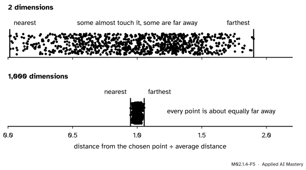
M02.1.4-F5
An experiment. Scatter 1,000 points at random in a cube and measure how far each lies from one more random point. In 2 dimensions the distances are spread widely. In 1,000 dimensions they are nearly all the same.
The experiment in the figure is run in the code below. In 2 dimensions the farthest point was about 136 times as far away as the nearest. In 1,000 dimensions it was only 1.11 times as far. When every point is about equally far away, “the nearest one” means much less. This is one face of what is called the curse of dimensionality, and a reason why intuition from the plane must be used with care in machine learning.
Worked example
Which house is most like house Q? The data are the five houses of the first figure.
House
Area (m²)
Bedrooms
A
104
5
B
112
2
C
60
1
D
160
3
Q
100
2
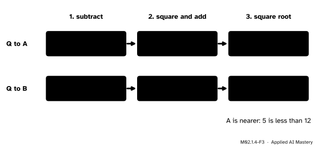
Step 1: distances in the units given. Subtract, square and add, take the root.
M02.1.4-F3
The distance from Q to A and from Q to B, in three steps each. In these units A is the nearer house.
\(\vect{a} - \vect{q} = (104 - 100,\; 5 - 2) = (4, 3)\), so \(\operatorname{dist}(\vect{a}, \vect{q}) = \sqrt{16 + 9} = 5\). And \(\vect{b} - \vect{q} = (12, 0)\), so \(\operatorname{dist}(\vect{b}, \vect{q}) = \sqrt{144 + 0} = 12\). Houses C and D are much further, at about 40.01 and 60.01. So the nearest house to Q is A, a house with five bedrooms where Q has two.
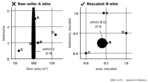
Step 2: change one unit. Measure area in hundreds of square metres. Now \(\vect{q} = (1.00, 2)\), \(\vect{a} = (1.04, 5)\) and \(\vect{b} = (1.12, 2)\). Then \(\operatorname{dist}(\vect{a}, \vect{q}) = \sqrt{0.04^2 + 3^2} = \sqrt{9.0016} \approx 3.0003\) and \(\operatorname{dist}(\vect{b}, \vect{q}) = \sqrt{0.12^2 + 0^2} = 0.12\). Now B is nearest. The houses have not changed. Only the unit has.
Step 3: rescale by the range. Areas run from 60 to 160, a range of 100. Bedrooms run from 1 to 5, a range of 4. By Fact 4,
Then \(\operatorname{dist}(\vect{a}', \vect{q}') = \sqrt{0.04^2 + 0.75^2} = \sqrt{0.5641} \approx 0.751\) and \(\operatorname{dist}(\vect{b}', \vect{q}') = \sqrt{0.12^2 + 0^2} = 0.12\). B is nearest, and by Fact 4 this answer would be the same in any units.
Code
Distance from scratch, then the three steps of the worked example with NumPy.
import numpy as npdef dist(a, b):"""Subtract, square, add, take the square root."""returnsum((x - y) **2for x, y inzip(a, b)) **0.5names = ["A", "B", "C", "D", "Q"]X = np.array([[104, 5], [112, 2], [60, 1], [160, 3], [100, 2]], dtype=float)q = X[4]print("raw units: ", [round(float(dist(row, q)), 2) for row in X[:4]])hundreds = X / np.array([100, 1]) # area in hundreds of square metresprint("area in 100 m²: ", np.linalg.norm(hundreds[:4] - hundreds[4], axis=1).round(4))low, high = X.min(axis=0), X.max(axis=0)scaled = (X - low) / (high - low) # min-max rescaling, Fact 4d_scaled = np.linalg.norm(scaled[:4] - scaled[4], axis=1)print("rescaled: ", d_scaled.round(3), " nearest:", names[int(np.argmin(d_scaled))])
raw units:       [5.0, 12.0, 40.01, 60.01]
area in 100 m²:  [3.0003 0.12   1.077  1.1662]
rescaled:        [0.751 0.12  0.472 0.65 ]  nearest: B
The library version of the rescaling is scikit-learn’s MinMaxScaler. The next cell checks that it agrees, then tries distance on real pictures: 1,797 handwritten digits of 8 by 8 pixels, each a vector in \(\R^{64}\).
from sklearn.datasets import load_digitsfrom sklearn.preprocessing import MinMaxScalerprint("same as MinMaxScaler:", np.allclose(MinMaxScaler().fit_transform(X), scaled))digits = load_digits()pictures, labels = digits.data, digits.targetagree =0for i, picture inenumerate(pictures): d = np.linalg.norm(pictures - picture, axis=1) d[i] = np.inf # a picture may not choose itself agree += labels[int(np.argmin(d))] == labels[i]print(pictures.shape, " nearest picture shows the same digit:", agree, "times out of", len(pictures))
same as MinMaxScaler: True
(1797, 64)  nearest picture shows the same digit: 1776 times out of 1797
For 1,776 of the 1,797 pictures, the closest other picture shows the same digit. Nothing here was trained. Distance between vectors did all the work. Last, the two high-dimensional facts.
print("cube diagonals:", [round(float(np.linalg.norm(np.ones(n))), 2) for n in (2, 3, 100, 784)])rng = np.random.default_rng(0)ratios = []for n in (2, 1000): points, chosen = rng.random((1000, n)), rng.random(n) d = np.linalg.norm(points - chosen, axis=1) ratios.append(round(float(d.max() / d.min()), 2))print(n, "dimensions: nearest", d.min().round(2), " farthest", d.max().round(2), " ratio", ratios[-1])
This module’s interactive, the vector playground, lives in lesson M02.1.3. Switch on Show v − u there: the length of that arrow is the distance between the two tips, which is the distance of this lesson.
Pitfalls
M02.1.4-F4
Wrong beside right. Both plots show the same houses, and the shaded region is “everything as close to Q as its nearest neighbour”. In raw units that region is a tall sliver that reaches A. After rescaling it is a circle, and the neighbour is B.
“Distance is distance. The units cannot matter.”
They decide the answer. In square metres, the nearest house to Q was A. In hundreds of square metres it was B. The formula adds up squared differences without knowing what they measure, so the feature with the biggest numbers wins. Rescale the features before using distance, and learn the rescaling from the data you train on.
“Any numbers will do as features, so I will code red, green and blue as 1, 2 and 3.”
That invents an order and a spacing that the colours do not have. With those codes, red is at distance 1 from green and at distance 2 from blue, so the computer believes red is more like green. A common fix is one coordinate per colour: red \(= (1, 0, 0)\), green \(= (0, 1, 0)\), blue \(= (0, 0, 1)\). Now every pair is at the same distance, \(\sqrt{1 + 1 + 0} = \sqrt{2}\).
“A space with 1,000 dimensions is like ordinary space, with more axes.”
In some ways it is not. A cube with sides of length 1 has a diagonal of length \(\sqrt{1000} \approx 31.6\), and in the experiment above the nearest of 1,000 random points was almost as far away as the farthest. Methods that lean on “the nearest few points” need more care as the dimension grows.
“King minus man plus woman equals queen.”
In the toy picture, exactly. In a real embedding the sum lands near the vector for queen, and “queen” is the answer only because it is the closest word to that spot. The arithmetic of lesson M02.1.3 still applies. What it returns is a point, and the nearest word has to be searched for.
Check yourself
Recall
1. What is a feature vector?
Show answer
The list of an object’s measurements (its features), written in a fixed order. It is a vector in \(\R^n\), where \(n\) is the number of features.
2. How is the distance between two data points \(\vect{a}\) and \(\vect{b}\) computed?
Show answer
It is the length of their difference, \(\norm{\vect{a} - \vect{b}}\): subtract coordinate by coordinate, square, add, and take the square root.
3. One feature is switched to a unit 10 times smaller. What happens to its term in the squared distance?
Show answer
Its values are multiplied by 10, so its term is multiplied by \(10^2 = 100\). The other terms do not change.
4. What does min-max rescaling do to a feature?
Show answer
It subtracts the smallest value and divides by the range, \(x' = (x - m)/(M - m)\), so that the feature runs from 0 to 1 whatever unit it was measured in.
5. How long is the diagonal of the cube with sides of length 1 in \(\R^n\)?
Show answer
\(\sqrt{n}\): the distance from \((0, \dots, 0)\) to \((1, \dots, 1)\).
Exercises
1.★ A picture has 2 rows and 3 columns of pixels. Its top row holds \(0, 1, 1\) and its bottom row holds \(1, 0, 0.5\). Write it as a vector, state its dimension, and find its distance from the blank picture, in which every pixel is 0.
Show solution
Row by row, the vector is \((0, 1, 1, 1, 0, 0.5)\). It has 6 coordinates, so it is in \(\R^6\). Its distance from \((0, 0, 0, 0, 0, 0)\) is \(\sqrt{0 + 1 + 1 + 1 + 0 + 0.25} = \sqrt{3.25} \approx 1.80\).
2.★★ Songs are described by (tempo in beats per minute, loudness from 0 to 1). In a collection, tempo runs from 80 to 180 and loudness from 0.1 to 0.9. Three of the songs are \(X = (120, 0.9)\), \(Y = (124, 0.1)\) and \(Z = (140, 0.8)\). Which of \(Y\) and \(Z\) is nearer to \(X\) (a) in these units and (b) after min-max rescaling?
Show solution
(a) \(\operatorname{dist}(X, Y) = \sqrt{4^2 + 0.8^2} = \sqrt{16.64} \approx 4.08\) and \(\operatorname{dist}(X, Z) = \sqrt{20^2 + 0.1^2} = \sqrt{400.01} \approx 20.00\). \(Y\) is nearer, although it is a quiet song and \(X\) is a loud one.
(b) Tempo has range 100 and loudness has range 0.8, so \(X' = \big(\tfrac{40}{100}, \tfrac{0.8}{0.8}\big) = (0.40, 1)\), \(Y' = \big(\tfrac{44}{100}, \tfrac{0}{0.8}\big) = (0.44, 0)\) and \(Z' = \big(\tfrac{60}{100}, \tfrac{0.7}{0.8}\big) = (0.60, 0.875)\). Then \(\operatorname{dist}(X', Y') = \sqrt{0.04^2 + 1^2} = \sqrt{1.0016} \approx 1.001\) and \(\operatorname{dist}(X', Z') = \sqrt{0.2^2 + 0.125^2} = \sqrt{0.055625} \approx 0.236\). Now \(Z\) is nearer.
3.★★★ Show that sliding every data point by the same vector \(\vect{w}\) changes no distance, and that scaling every data point by the same number \(c\) multiplies every distance by \(\abs{c}\). Why does the second fact not contradict Fact 3?
Show solution
Sliding. Coordinate \(i\) of \((\vect{a} + \vect{w}) - (\vect{b} + \vect{w})\) is \((a_i + w_i) - (b_i + w_i) = a_i - b_i\), so \((\vect{a} + \vect{w}) - (\vect{b} + \vect{w}) = \vect{a} - \vect{b}\). The two differences are the same vector, so they have the same length: \(\operatorname{dist}(\vect{a} + \vect{w}, \vect{b} + \vect{w}) = \operatorname{dist}(\vect{a}, \vect{b})\).
Scaling. Write \(\vect{d} = \vect{a} - \vect{b}\). By rules 6 and 7 of lesson M02.1.3, \(c\vect{a} - c\vect{b} = c\vect{d}\). Then
No contradiction. Here every coordinate is scaled by the same number, so every distance is multiplied by the same \(\abs{c}\) and the nearest point stays the nearest. In Fact 3 only one coordinate is scaled. That changes some distances more than others, and the ranking can change.
Summary card
Describe each object by a list of numbers and it becomes a point: likeness becomes distance.
M02.1.4-F1
Rows become points.
Feature vector. An object’s measurements in a fixed order: a vector in \(\R^n\).
Distance.\(\operatorname{dist}(\vect{a}, \vect{b}) = \norm{\vect{a} - \vect{b}}\): subtract, square, add, take the root.
Units matter. A unit \(s\) times smaller makes that feature count \(s^2\) times more.
Rescale first.\(x' = (x - m)/(M - m)\) puts every feature on the range 0 to 1.
High dimensions. The unit cube’s diagonal is \(\sqrt{n}\), and random points become almost equally far apart.
Sources and next steps
Sources. Each was opened and checked against this lesson on 12 November 2026.
Stephen Boyd and Lieven Vandenberghe, Introduction to Applied Linear Algebra: Vectors, Matrices, and Least Squares (free PDF). Section 1.1 gives feature vectors, images as vectors of pixel values and word-count vectors as examples. Section 3.2 defines the distance as the norm of the difference, describes feature distance and the nearest neighbour, and under “Units for heterogeneous vector entries” explains with a house example (area and bedrooms) why units must be chosen so that entries have similar sizes.
Tomas Mikolov, Kai Chen, Greg Corrado and Jeffrey Dean, Efficient Estimation of Word Representations in Vector Space (2013). Section 1.1 reports that vector(“King”) − vector(“Man”) + vector(“Woman”) results in a vector that is closest to the vector for the word Queen. Its tables compare word vectors with 300 and 640 coordinates.
Pedro Domingos, A Few Useful Things to Know about Machine Learning, Communications of the ACM 55(10), 2012. The section “Intuition fails in high dimensions” describes the curse of dimensionality and says that intuitions from a three-dimensional world often do not apply in high-dimensional ones.
scikit-learn User Guide, Preprocessing data. The sections on standardisation and on scaling features to a range give the MinMaxScaler formula used in Fact 4 and warn that a feature with a much larger spread can dominate.
scikit-learn, load_digits. The digits data used in the code: 1,797 samples, each an 8 by 8 image, 64 features.
Next. Module M02.2 begins with M02.2.1, Linear combinations: scaling and adding rolled into one operation. Module M02.3 returns to length and distance and adds angles to the picture.