Compare every pair of groups after an ANOVA with Tukey’s honestly significant difference, worked on rent by district, then meet multiplicity where data scientists meet it: many metrics in one experiment, feature screens over thousands of columns, and leaderboards reused until they overfit.
S02.9.4L2 Intermediate25 minIn review (what this means)
The maths and code on this page are checked by automated tests on every change, but an independent reader has not signed it off yet. Spot a mistake or a confusing step? Tell us.
Compute Tukey’s honestly significant difference from the within-group mean square and the studentized range, and use it to compare every pair of group means.
Explain why picking the largest gap and then testing it needs the range distribution, not a plain t-test.
Choose a correction for many metrics in one experiment and for a feature screen, using Holm, scikit-learn’s SelectFwe and SelectFdr.
Describe how a reused holdout overfits, and list the defences: fix the analysis first, keep a fresh test set, correct for the tests run and report how many were run.
The question
The ANOVA of S02.7.3 asked one question of the nine flats: do the three districts share a mean rent? Now you want to know which districts differ: three pairs, three tests, and a family-wise error to protect. The same question comes back in every data team: one experiment with twelve metrics, a screen of a thousand features, a leaderboard checked after every submission. How is each one kept honest?
From the last lesson
1. How many of the ten p-values does Benjamini-Hochberg reject at \({q = 0.05}\)?
Show answer
Three: 0.001, 0.008 and 0.012, the largest rank under the line \({0.005\,k}\) being 3.
2. What does an FDR of 0.05 promise?
Show answer
That the share of false discoveries among the discoveries is at most 0.05 on average over repetitions of the study, not in every list.
Intuition
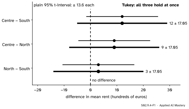
Three districts give three pairs, and three plain 95 percent intervals each miss 5 percent of the time. Tukey’s idea is to widen all of them by the same amount, just enough that all three hold at once 95 percent of the time. One number, the honestly significant difference, sets the width.
S02.9.4-F1
Pairwise differences of mean rent for the nine flats of S01 (invented). Tukey’s intervals (thick) are wider than the plain ones (thin) so that all three cover their true differences together 95 percent of the time. Every interval contains 0.
Build it up
Step 1. Count the pairs.\(k\) groups give \({k(k - 1)/2}\) pairs: 3 for three groups, 10 for five, 45 for ten. The family grows with the square of the number of groups.
Step 2. One pair, one t. ANOVA’s within-group mean square estimates the shared variance: \({MS_W = 278/6} = 46.33\) on 6 degrees of freedom. With three flats per district the standard error of a difference of two means is \({\sqrt{46.33 \times 2/3}} = 5.56\), and the plain interval is \({\pm\, 2.447 \times 5.56} = {\pm\, 13.6}\).
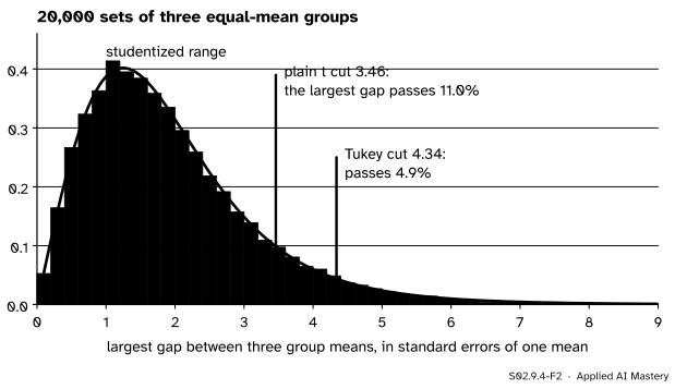
Step 3. All pairs at once. No pair is declared different exactly when even the largest gap between two means is too small. The largest gap is the range of the means. Measured in standard errors of one mean, \({\sqrt{MS_W/n}}\), it has a known distribution under equal means, the studentized range.
S02.9.4-F2
Under equal means (seed 3), the largest of the three gaps clears the plain t cut-off 11 percent of the time, more than twice the promised 5. The 95th percentile of the studentized range, 4.34, brings it back to 5.
Step 4. The cut-off. The 95th percentile of the studentized range for 3 means and 6 degrees of freedom is \({Q_{3,6,\,0.95}} = 4.339\). Multiply by the standard error of one mean: \({4.339 \times 3.93} = 17.05\), the honestly significant difference.
The formal statement
NoteTukey’s honestly significant difference
For \(k\) groups of \(n\) values each, with within-group mean square \(MS_W\) on \({N - k}\) degrees of freedom, let \({Q_{k,N-k,\,1-\alpha}}\) be the \({1 - \alpha}\) quantile of the studentized range. Declare groups \(g\) and \(h\) different when
Equivalently, the intervals \({\bar x_g - \bar x_h \pm \text{HSD}}\) cover all the true differences at once with probability \({1 - \alpha}\).
The studentized range is written \(Q\) here because \(q\) is the FDR level. With equal group sizes and normal data of one variance, the family-wise level is exactly \(\alpha\) when all means are equal, and the simultaneous coverage is exactly \({1 - \alpha}\). With unequal sizes the Tukey-Kramer version uses each pair’s own standard error, and its coverage is at least \({1 - \alpha}\).
Why it beats Bonferroni. In units of the standard error of a difference, Tukey’s multiplier is \({4.339/\sqrt 2} = 3.07\). Bonferroni would test each of the 3 pairs at level \({0.05/3}\) and use \({t_{6,\,1 - 0.05/6}} = 3.29\). Tukey is narrower because it uses the exact joint distribution of the three gaps, which share data, where Bonferroni only bounds it.
Many metrics in one experiment. An A/B test that watches twelve metrics is a family of twelve. The usual defence is to name one primary metric before the test starts and judge the experiment on it alone at level \(\alpha\). Secondary metrics are corrected, with Holm if any one false claim matters, and guardrail metrics, which only check that nothing broke, are reported separately (S05.2).
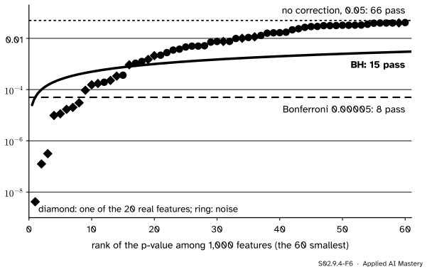
Feature screens. Testing each of thousands of columns against a label is the textbook FDR setting: many real signals may exist, and a few false leads are tolerable before a model is fitted. scikit-learn’s SelectFdr applies Benjamini-Hochberg to the p-values of f_classif, and SelectFwe applies a Bonferroni cut-off.
S02.9.4-F6
A screen of 1,000 features of which 20 are real (seed 0). Without correction 66 pass and 46 of them are noise; BH keeps 15 with 2 false; Bonferroni keeps 8, none false.
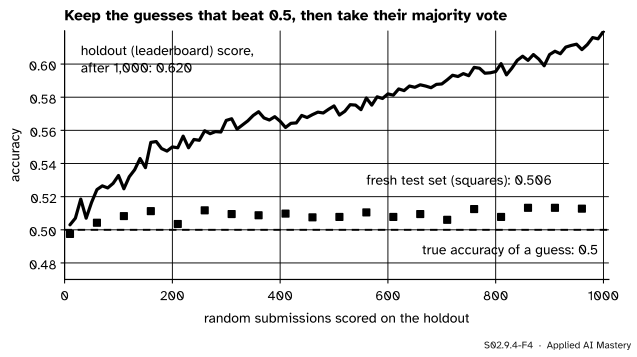
Leaderboards. A held-out set that is scored again and again stops being held out: each score is a test, and the choices that follow it are fitted to the holdout. Blum and Hardt’s boosting attack shows how far this goes. Submit random guesses, keep those that score above 0.5 on the holdout, and take their majority vote. Nothing has been learned, yet the holdout score climbs.
S02.9.4-F4
The boosting attack on a holdout of 4,000 random labels (seed 0). After 1,000 guesses the leaderboard reads 0.620; a fresh test set reads 0.506, chance.
The defences, each a way to keep the family small or to pay for it:
Fix the analysis before seeing the data: the outcome, the test, the exclusions.
Keep a test set that is used once, at the end (ML01.9.4).
Correct for every test that was actually run, not only those reported.
Report how many tests and analyses were run, as S01.8.4 asks of every report (S01.8.4).
Worked example
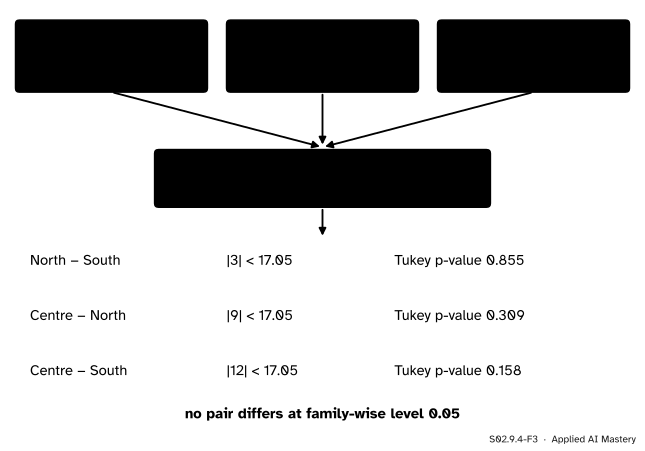
Which districts differ? South 3, 8, 4; North 7, 10, 7; Centre 12, 30, 9; means 5, 8 and 17.
S02.9.4-F3
Tukey’s method on the nine flats, from the ANOVA’s within mean square to a verdict on every pair.
From the ANOVA: \({MS_W = 278/6} = 46.33\) on \({9 - 3} = 6\) degrees of freedom.
Standard error of one district mean: \({\sqrt{46.33/3}} = {\sqrt{15.44}} = 3.93\).
Studentized range quantile for 3 means and 6 degrees of freedom: \({Q_{3,6,\,0.95}} = 4.339\) (from scipy.stats.studentized_range.ppf).
HSD: \({4.339 \times 3.93} = 17.05\).
Gaps: \({8 - 5} = 3\), \({17 - 8} = 9\), \({17 - 5} = 12\). All are below 17.05, so no pair differs at family-wise level 0.05. The Tukey p-values are 0.855, 0.309 and 0.158.
This agrees with the ANOVA’s p-value of 0.160: three flats per district and one penthouse leave too much noise to separate any two districts.
Code
Tukey from scratch with the studentized range, then scipy.stats.tukey_hsd.
import itertoolsimport numpy as npfrom scipy import statsrents = {"South": [3, 8, 4], "North": [7, 10, 7], "Centre": [12, 30, 9]} # S01's flats (invented)k, n =len(rents), 3ms_w =sum(((np.array(v) - np.mean(v)) **2).sum() for v in rents.values()) / (k * n - k)se_mean = np.sqrt(ms_w / n)Q = stats.studentized_range.ppf(0.95, k, k * n - k)print(f"MS_W = {ms_w:.2f}, se = {se_mean:.2f}, Q = {Q:.3f}, HSD = {Q * se_mean:.2f}")ours = {}for a, b in itertools.combinations(rents, 2): gap =abs(np.mean(rents[a]) - np.mean(rents[b])) ours[(a, b)] = stats.studentized_range.sf(gap / se_mean, k, k * n - k)print(f"{a} vs {b}: gap {gap:.0f}, Tukey p-value {ours[(a, b)]:.3f}")res = stats.tukey_hsd(*rents.values())print(res.pvalue.round(3))print("interval half-width:", (res.confidence_interval().high - res.statistic)[0, 1].round(2))
MS_W = 46.33, se = 3.93, Q = 4.339, HSD = 17.05
South vs North: gap 3, Tukey p-value 0.855
South vs Centre: gap 12, Tukey p-value 0.158
North vs Centre: gap 9, Tukey p-value 0.309
[[1.    0.855 0.158]
 [0.855 1.    0.309]
 [0.158 0.309 1.   ]]
interval half-width: 17.05
The chance that the largest of the three gaps clears the plain t cut-off under equal means is studentized_range.sf at \({\sqrt 2 \times 2.447}\): 0.109. Now a feature screen: 200 examples, 1,000 features, the first 20 shifted by 0.6 in one class.
SelectFdr keeps exactly the features that false_discovery_control passes. Finally the boosting attack, with 1,000 random guesses at 4,000 random holdout labels.
rng = np.random.default_rng(0)holdout = rng.integers(0, 2, 4000)fresh = rng.integers(0, 2, 4000) # new labels the guesses never sawguesses = rng.integers(0, 2, (1000, 4000))lucky = guesses[(guesses == holdout).mean(1) >0.5] # keep the guesses that beat 0.5vote = (lucky.mean(0) >0.5).astype(int)print(f"kept {len(lucky)}; holdout accuracy {np.mean(vote == holdout):.3f}, fresh {np.mean(vote == fresh):.3f}")
kept 525; holdout accuracy 0.620, fresh 0.506
Explore
The many-tests simulator is in lesson S02.9.3. Treat it as a feature screen: 200 tests with 10 percent real effects of size 3. Compare the uncorrected count, which is padded with noise, with BH’s, and see how few Bonferroni keeps.
Pitfalls
S02.9.4-F5
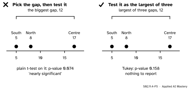
Wrong beside right. Choosing the biggest gap after looking and testing it alone gives 0.074. The gap was chosen as the largest of three, and Tukey’s p-value for that is 0.158.
“I only tested the one pair that looked different.”
Looking chose it, and looking compared all three pairs. Under equal means the largest gap clears the plain cut-off 10.9 percent of the time, not 5. Tukey’s method is the test of the comparison you actually made.
“Three of our twelve metrics moved, so the change works.”
With twelve metrics at 0.05 and no effect at all, a false mover turns up in \({1 - 0.95^{12}} = 46\) percent of experiments, if the metrics were independent. Decide on the primary metric in advance; correct the others, or call them exploratory.
“Our validation score is honest: we never trained on the validation set.”
Choosing on it is a kind of training. A holdout scored after every change overfits just as the boosting attack shows, slowly and without anyone cheating. Keep a test set that is opened once.
Check yourself
Recall
1. How many pairwise comparisons do \(k\) groups give, and how many for six?
Show answer
\({k(k - 1)/2}\); for six groups, 15.
2. What is the studentized range, and why does Tukey’s method use it?
Show answer
The range of \(k\) group means divided by the estimated standard error of one mean. No pair is declared different exactly when the largest gap is small enough, so the range’s distribution gives the cut-off that holds the family-wise level at \(\alpha\).
3. What is the honestly significant difference for rent by district, and which pairs exceed it?
Show answer
\({4.339 \times 3.93} = 17.05\); none of the gaps 3, 9 and 12 exceeds it.
4. Which scikit-learn selectors apply Benjamini-Hochberg and a Bonferroni cut-off to feature p-values?
Show answer
SelectFdr applies Benjamini-Hochberg; SelectFwe applies a Bonferroni cut-off.
5. What does the boosting attack show?
Show answer
That a holdout scored many times can be fitted: keeping random guesses that beat 0.5 and voting lifts the holdout score (to 0.620 here) while accuracy on fresh data stays at chance.
Exercises
1.★ An experiment compares five page designs. How many pairwise comparisons are there, and what per-pair level would Bonferroni use for a family-wise 0.05?
Show solution
\({5 \times 4/2} = 10\) pairs, so Bonferroni tests each at \({0.05/10} = 0.005\). Tukey’s method, which uses the joint distribution of the gaps, is a little less strict.
2.★★ Lower the penthouse’s rent from 30 to 15, as in S02.7.3. The Centre becomes 12, 15, 9 with mean 12, and \({MS_W = 38/6}\). With \({Q_{3,6,\,0.95} = 4.339}\), which pairs differ?
Show solution
\({MS_W = 6.33}\), so the standard error of one mean is \({\sqrt{6.33/3}} = 1.453\) and \({\text{HSD} = 4.339 \times 1.453} = 6.30\). The gaps are \({8 - 5} = 3\), \({12 - 8} = 4\) and \({12 - 5} = 7\). Only Centre against South exceeds 6.30; its Tukey p-value is 0.033. The other two pairs do not differ.
3.★★★ Show that for two groups Tukey’s test is the pooled two-sample t-test: \({Q_{2,\nu,\,1-\alpha}} = {\sqrt 2\; t_{\nu,\,1-\alpha/2}}\).
Show solution
With two groups the range of the means is \({\abs{\bar x_1 - \bar x_2}}\), so
where \(t\) is the pooled two-sample statistic on \({\nu = 2n - 2}\) degrees of freedom. Then \({\Prob(Q > c)} = {\Prob(\abs{t} > c/\sqrt 2)}\), and setting this to \(\alpha\) gives \({c/\sqrt 2} = {t_{\nu,\,1-\alpha/2}}\). For \({\nu = 6}\): \({\sqrt 2 \times 2.447} = 3.460\), which is studentized_range.ppf(0.95, 2, 6).
Summary card
Count the tests you could have run, and pay for them.
S02.9.4-F1
Tukey: all three pairs at once.
Tukey. Differ when \({\abs{\bar x_g - \bar x_h}} > {Q_{k,N-k,\,1-\alpha}\sqrt{MS_W/n}}\).
Metrics. One primary metric fixed in advance; correct or label the rest.
Screens. FDR control: SelectFdr is Benjamini-Hochberg.
Holdouts. Reuse overfits; keep a test set opened once, and report how many tests were run.
Sources and next steps
Sources. Each was opened and checked against this lesson on 15 November 2026.
NIST/SEMATECH, e-Handbook of Statistical Methods, Section 7.4.7.1, Tukey’s method: the studentized range \({q(r, \nu) = w/s}\), the simultaneous intervals for all pairwise differences, exact confidence \({1 - \alpha}\) for equal sample sizes, and the conservative Tukey-Kramer method for unequal ones.
SciPy developers, scipy.stats.tukey_hsd: its assumptions (independence, normality, equal variances), the pvalue matrix and the confidence_interval() method with level 0.95 by default, and Tukey-Kramer for unequal sizes.
scikit-learn developers, sklearn.feature_selection.SelectFdr: “This uses the Benjamini-Hochberg procedure”, with f_classif as the default score function, and SelectFwe listed as selection by family-wise error rate.
Avrim Blum and Moritz Hardt (2015), The Ladder: a reliable leaderboard for machine learning competitions. Section 5 describes the boosting attack (random submissions, keep those with loss at most one half, coordinate-wise majority vote) and shows that it inflates the public leaderboard.
Next. Module S02.10, Likelihood theory: Fisher information and asymptotics, returns to the likelihood to explain where the large-sample tests of this course come from. Experiment design, primary metrics and guardrails are taken up in S05.2.