Numerical maximum likelihood and losses as likelihoods
When the score equation has no closed form, search for the peak: fit a gamma to 40 city rents with Newton’s method from a method-of-moments start, then with SciPy. Then see that minimising a mean negative log-likelihood is maximum likelihood, so log loss and cross-entropy training are MLE.
S02.3.4L2 Intermediate30 minIn review (what this means)
The maths and code on this page are checked by automated tests on every change, but an independent reader has not signed it off yet. Spot a mistake or a confusing step? Tell us.
Derive the equation for the gamma shape, ln k - digamma(k) = ln x-bar - mean of ln x, and explain why it has no closed-form solution.
Solve it with Newton’s method from a method-of-moments start, and check the answer with scipy.optimize.minimize and scipy.stats.gamma.fit.
Show that minimising the mean negative log-likelihood is the same as maximising the likelihood, and recognise the log loss and cross-entropy as negative log-likelihoods.
Split the mean negative log-likelihood into an entropy and a KL divergence, and explain maximum likelihood as minimising an estimate of the KL divergence.
The question
The city’s rents (S01) are skewed to the right, and a gamma curve, with a shape \(k\) and a scale \(\theta\), follows that skew well. Write its log-likelihood, set the derivatives to zero, and the equation for \(k\) refuses to be solved by algebra. How do we find a peak that no formula reaches? And why does every classifier you train, by minimising a “loss”, end up doing exactly this?
From the last lesson
1. For design A’s times 4, 5, 7, 8, 11, what are the MLEs of \(\mu\) and \(\sigma^2\)?
Show answer
\({\hat{\mu} = 7}\) and \({\hat{\sigma}^2 = 30/5 = 6}\), against \({s^2 = 30/4 = 7.5}\).
2. Under which noise model is least squares the maximum likelihood fit of a line?
Show answer
Independent normal errors of the same variance around the line.
Intuition
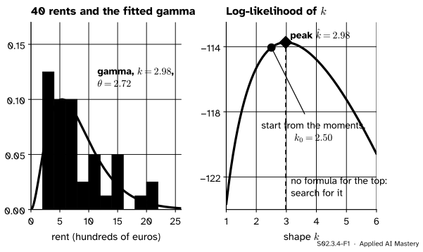
Draw 40 flats from the city of S01 and fit a gamma. For each shape \(k\) the best scale can be written down, so the log-likelihood becomes a curve in \(k\) alone. It has one clear peak. We cannot write the peak’s position as a formula, but we can climb to it: start near the top and take steps that home in on it.
S02.3.4-F1
Left: 40 rents drawn from the city (seed 1) and the maximum likelihood gamma. Right: the log-likelihood of the shape \(k\), with the scale at its best value for each \(k\). The method of moments (S02.2.4) starts the search close to the top, at 2.50; the top is at 2.98.
The same picture explains the second half of the lesson. Turn the curve upside down and divide by the number of rents, and it becomes a loss to minimise. Every “minimise the loss” in machine learning that uses log loss or cross-entropy is this climb, seen from below.
Build it up
Step 1. The gamma log-likelihood. The gamma density with shape \({k > 0}\) and scale \({\theta > 0}\) is
Step 2. The scale has a formula. Hold \(k\) fixed: \({\pd{\ell}{\theta} = \sum x_i / \theta^2 - nk/\theta}\). Setting it to zero gives \({\theta = \bar{x}/k}\): for each shape, the best scale makes the mean \({k\theta}\) equal \(\bar{x}\).
Step 3. The shape does not. With \({\psi(k) = \Gamma'(k)/\Gamma(k)}\), the digamma function,
where \(\overline{\ln x}\) is the mean of the logged data. The right-hand side is a number we can compute from the data, \({0.1771}\) for the 40 rents. The left-hand side mixes a logarithm with digamma, and no algebra isolates \(k\).
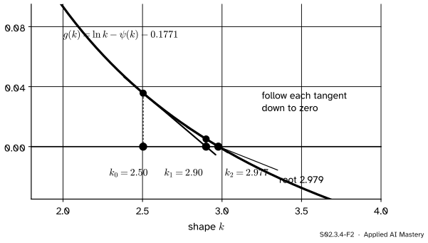
Step 4. Newton’s method. Call the difference \({g(k) = \ln k - \psi(k) - 0.1771}\); we want its zero. Newton’s method (M04.4.4) replaces \(g\) by its tangent line at the current guess and jumps to where the tangent meets zero:
(\(\psi'\) is the trigamma function, scipy.special.polygamma(1, k).)
Step 5. A good start. The gamma has mean \({k\theta}\) and variance \({k\theta^2}\). Matching them to the sample mean and the variance \(v\) (divisor \(n\)) gives the method-of-moments start \({k_0 = \bar{x}^2 / v}\) (S02.2.4).
S02.3.4-F2
Newton’s method on \({g(k) = \ln k - \psi(k) - 0.1771}\). From the moments start 2.50 the first tangent lands at 2.90, the second at 2.977, already next to the root 2.979.
The formal statement
NoteLosses as likelihoods
For a model with density (or probability) \(f(x \mid \theta)\) and independent data \({x_1, \dots, x_n}\), the mean negative log-likelihood is
Multiplying by \({-1/n}\) turns every peak of \(\ell\) into a valley of \(L\) at the same \(\theta\), so minimising \(L\) is maximum likelihood.
Three losses of this course are of this form.
Squared error. Under the model “normal around a line” (S02.3.3), \(L\) is a constant plus \({\tfrac{1}{2\sigma^2}}\) times the mean squared residual.
Log loss. A classifier that gives example \(i\) the probability \(p_i\) of the positive class is a Bernoulli model for the label \({y_i \in \{0, 1\}}\). The probability of the observed label is \({p_i^{y_i}(1 - p_i)^{1 - y_i}}\), so
the log loss of ML01.6.2. Training logistic regression is maximum likelihood.
Cross-entropy. With more than two classes, a network that outputs a probability for each class is a categorical model, and the mean of \({-\ln}\) (probability of the true class) is the cross-entropy loss of deep learning (DL01.4).
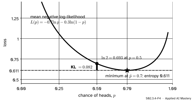
Maximum likelihood and the KL divergence. Take the coin again. Its data say “heads 0.7 of the time, tails 0.3”, and the mean negative log-likelihood of a model \(p\) is
The first part does not depend on \(p\). The second is the Kullback-Leibler divergence from the data’s proportions to the model’s (M09.3); it is never negative and is zero only when \({p = 0.7}\). So maximum likelihood picks the model closest to the data in the KL sense.
S02.3.4-F4
The coin’s mean negative log-likelihood as a loss. Its floor is the entropy of the data’s own proportions, 0.611, reached at \({\hat{p} = 0.7}\). At any other \(p\) the loss is higher by the KL divergence: 0.082 at \({p = 0.5}\).
With continuous data the same holds in the limit. By the law of large numbers (M06.11), \(L(\theta)\) tends to the expected value \({-\E[\ln f(X \mid \theta)]}\) under the true distribution, which is a constant plus the KL divergence from the truth to the model. Maximum likelihood minimises an estimate of that divergence. When the model family does not contain the truth, as with a single gamma for the city’s three districts, the MLE settles, as the sample grows, on the member of the family closest to the truth in KL divergence.
Worked example
Fit a gamma to the 40 rents. Their mean is \({\bar{x} = 8.0997}\) and their variance (divisor \(n\)) is \({v = 26.201}\), both in hundreds of euros. The mean of their logs is 1.9147.
S02.3.4-F3
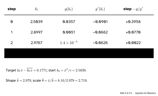
Newton’s method for the shape, step by step. The value of \(g\) shrinks from 0.036 to about \({10^{-7}}\) in three steps; each step roughly squares the error.
Target.\({\ln\bar{x} - \overline{\ln x}}\) is \({\ln 8.0997 - 1.9147}\), which is \({2.0918 - 1.9147}\) = 0.1771.
Start.\({k_0 = 8.0997^2 / 26.201 = 2.504}\).
Step 1.\({g(2.504) = 0.0357}\) and \({g'(2.504) = -0.0901}\), so \(k_1 = 2.504 + 0.0357/0.0901 = 2.900\).
Steps 2 and 3.\({k_2 = 2.9767}\) and \({k_3 = 2.9789}\), after which the digits stop changing.
Gain. The log-likelihood rises from \(-114.05\) at the start to \(-113.74\) at the peak: the method of moments was close, and maximum likelihood finishes the job.
Code
From scratch: the city, the sample of 40, and Newton’s method. scipy.special supplies digamma and trigamma.
import numpy as npfrom scipy import specialrng = np.random.default_rng(0) # the city of S01, built the course's wayparts = []for size, mean in ((250, 5), (150, 8), (100, 17)): draws = rng.gamma(9.0, 1.0, size) parts.append(draws * mean / draws.mean())city = np.concatenate(parts)x = np.random.default_rng(1).choice(city, 40, replace=False)target = np.log(x.mean()) - np.mean(np.log(x))k = x.mean() **2/ x.var() # method-of-moments start, divisor nsteps = [k]for _ inrange(4): g = np.log(k) - special.digamma(k) - target slope =1/ k - special.polygamma(1, k) k = k - g / slope steps.append(k)k_hat, theta_hat = steps[-1], x.mean() / steps[-1]print("mean", round(x.mean(), 4), " variance", round(x.var(), 3), " target", round(target, 4))print("Newton:", [round(float(s), 4) for s in steps])print("k =", round(float(k_hat), 3), " theta =", round(float(theta_hat), 3))
mean 8.0997  variance 26.201  target 0.1771
Newton: [2.5039, 2.8997, 2.9767, 2.9789, 2.9789]
k = 2.979  theta = 2.719
Two library routes to the same peak. scipy.optimize.minimize minimises the negative log-likelihood; searching over \({\ln k}\) and \({\ln\theta}\) keeps both parameters positive. scipy.stats.gamma.fit does maximum likelihood by default; floc=0 fixes SciPy’s extra location parameter at 0, the model of this lesson.
minimize:  k 2.979  theta 2.719  ell -113.74
gamma.fit: k 2.979  theta 2.719
ell at the moments start: -114.05
Now losses. scikit-learn’s log_loss is the mean negative log-likelihood of Bernoulli labels: for the coin it is \({-\ell(0.7)/10}\), and for the six students of ML01.6.2 under the model \({p = \sigma(x - 3.5)}\) it is the 0.418 of that lesson.
coin: log loss 0.6109  -ell/n 0.6109  KL at 0.5: 0.0823
students: log loss 0.418  -ell/n 0.418
At the MLE the coin’s log loss equals the entropy exactly, and the gap at \({p = 0.5}\) is the KL divergence, as the formal section derived.
Explore
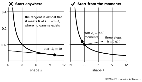
The module’s interactive, the likelihood surface explorer, is in lesson S02.3.3. Go back to it with this lesson in mind: the contour map there is a loss map seen upside down, and the peak is where an optimiser minimising the mean negative log-likelihood would stop. In the code above, try starting Newton’s method at \({k = 10}\) instead of the moments start and see what happens to the next step.
Pitfalls
S02.3.4-F5
Wrong beside right. From \({k = 10}\), where \(g\) is almost flat, the tangent sends Newton’s method to \({k = -14.4}\), outside the allowed shapes, and the next step fails. From the method-of-moments start it converges in three steps.
“Newton’s method always finds the root; the start does not matter.”
Newton’s method trusts the tangent line, which is a good guide only near the root. Far away, where \(g\) is nearly flat, one step can throw the guess out of the allowed range, as here, or to a different flat point. Start close (the method of moments is cheap and usually close), keep the parameters in range by working with \({\ln k}\), or fall back on a safer method such as bisection.
“The fitted gamma is the distribution of the city’s rents.”
Maximum likelihood finds the best member of the family you chose, not the truth. The city’s rents are a mix of three districts, each with its own scale, so no single gamma is exactly right. The fit is the gamma that makes these 40 rents most probable, an estimate of the gamma closest to the city in the KL sense. Check it, for example by comparing the fitted curve with a histogram (S01.4), before trusting its tail.
“A loss is a choice of taste; the likelihood is a separate, statistical idea.”
For the losses that train most models they are the same object. Log loss is the Bernoulli negative log-likelihood, cross-entropy is the categorical one, and squared error is the normal one. Choosing a loss is choosing a noise model, and a model trained this way is a maximum likelihood estimate, with the strengths and the biases of one.
Check yourself
Recall
1. What equation does the MLE of the gamma shape solve, and why is a numerical method needed?
Show answer
\({\ln k - \psi(k) = \ln\bar{x} - \overline{\ln x}}\). The digamma function \(\psi\) cannot be inverted together with \(\ln k\) by algebra, so the root is found by a search such as Newton’s method.
2. What is the Newton step for solving \({g(k) = 0}\)?
Show answer
\({k_{t+1} = k_t - g(k_t)/g'(k_t)}\): follow the tangent line at \(k_t\) to where it meets zero.
3. Why start from the method of moments?
Show answer
It is a quick formula, \({k_0 = \bar{x}^2/v}\), that lands close to the MLE (2.50 against 2.98 for the rents), and Newton’s method is reliable when it starts close.
4. Why is minimising the mean negative log-likelihood the same as maximum likelihood?
Show answer
\({L = -\ell/n}\), and multiplying by the negative number \({-1/n}\) turns the highest point of \(\ell\) into the lowest point of \(L\) at the same parameter.
5. Which likelihood is the log loss of logistic regression?
Show answer
The Bernoulli likelihood of the labels, with probability \(p_i\) of a positive label for example \(i\): log loss is its mean negative logarithm.
Exercises
1.★ Three classes have predicted probabilities 0.7, 0.2, 0.1 for one example whose true class is the second. What is its cross-entropy loss? What would it be if the model gave the true class probability 0.9?
Show solution
The loss is \({-\ln}\) of the probability of the true class: \({-\ln 0.2 = 1.609}\). With 0.9 it would be \({-\ln 0.9 = 0.105}\). The other probabilities do not enter, except through the requirement that all three add to 1.
2.★★ Use Newton’s method on \({h(\lambda) = 5/\lambda - 10}\), the score of the waiting times of S02.3.2, starting at \({\lambda_0 = 0.4}\). Do two steps. Then try \({\lambda_0 = 1.2}\).
From 0.4: \({0.8 - 0.32 = 0.48}\), then \({0.96 - 0.4608 = 0.4992}\), closing in on 0.5. From 1.2: \({2.4 - 2.88 = -0.48}\), a negative rate, which is impossible. The same lesson as the gamma: start close. Here any start strictly between 0 and 1 converges to 0.5, because \({2\lambda(1 - \lambda)}\) then lies between 0 and 0.5; a start at 1 or beyond does not.
3.★★★ Show that for any data the mean negative log-likelihood of a coin model \(p\), with observed share of heads \(\hat{p}\), is \({H(\hat{p}) + \mathrm{KL}(\hat{p}, p)}\), and that the KL part is never negative. (Use \({\ln u \le u - 1}\).)
Show solution
With \(k\) heads in \(n\) tosses, \({L(p) = -\hat{p}\ln p - (1 - \hat{p})\ln(1 - p)}\). Adding and subtracting \({\hat{p}\ln\hat{p} + (1 - \hat{p})\ln(1 - \hat{p})}\) splits it into \({H(\hat{p}) = -\hat{p}\ln\hat{p} - (1 - \hat{p})\ln(1 - \hat{p})}\) and
So \({\mathrm{KL} \ge 0}\), with equality only when \({p = \hat{p}}\), which is again the MLE. (If \(\hat{p}\) is 0 or 1, the terms with a zero weight are left out.)
Summary card
No formula? Search. Minimising a log loss is maximising a likelihood.
S02.3.4-F1
Start at the moments, climb to the peak.
Gamma shape.\({\ln k - \psi(k) = \ln\bar{x} - \overline{\ln x}}\), then \({\hat{\theta} = \bar{x}/\hat{k}}\).
Newton.\({k_{t+1} = k_t - g(k_t)/g'(k_t)}\), from \({k_0 = \bar{x}^2/v}\): 2.979 for the 40 rents.
Losses.\({L(\theta) = -\ell(\theta)/n}\): log loss, cross-entropy and squared error are of this form.
KL.\({L = H + \mathrm{KL}}\): maximum likelihood is closest in KL divergence.
Sources and next steps
Sources. Each was opened and checked against this lesson on 15 November 2026.
Philippe Rigollet, Maximum Likelihood Estimation, MIT OpenCourseWare 18.650, Fall 2016, slides. The four slides on the Kullback-Leibler divergence write it as a constant minus the expected log-density, estimate that expectation by an average over the data (law of large numbers), and conclude that minimising the estimated divergence is maximising the likelihood: “the maximum likelihood principle”.
SciPy documentation, rv_continuous.fit: maximum likelihood is the default method (method of moments is the alternative), it minimises the negative log-likelihood, and floc holds the location fixed; scipy.special.digamma: the logarithmic derivative of the gamma function; scipy.optimize.minimize: minimisation of a scalar function of several variables, with the Nelder-Mead method among others.
scikit-learn documentation, sklearn.metrics.log_loss: log loss, also called logistic loss or cross-entropy loss, the loss of logistic regression and of neural networks, defined as the negative log-likelihood of a logistic model that returns probabilities for its training data.
Jeremy Orloff and Jonathan Bloom, Reading 10b: Maximum Likelihood Estimates, MIT OpenCourseWare 18.05, Spring 2022: the definition of the MLE that every fit in this lesson computes.
Next. Course S02 goes on to S02.4 Confidence intervals, which asks how far an estimate is likely to be from the truth. The precision of the MLE itself, read from the curvature of the log-likelihood at its peak, is S02.10.