The p-value is the chance, if the null hypothesis were true, of a result at least as extreme as the one observed. Compute it one- and two-sided, run a z-test with math.erf, prove that under the null it is uniform, and learn what it does not measure.
S02.5.2L2 Intermediate25 minIn review (what this means)
The maths and code on this page are checked by automated tests on every change, but an independent reader has not signed it off yet. Spot a mistake or a confusing step? Tell us.
Define the p-value and compute it one-sided and two-sided for a binomial count (0.172 and 0.344 for the coin).
Run a z-test for a mean with a known standard deviation, taking its p-value from Φ written with math.erf.
Prove that the p-value of a continuous statistic is uniform on [0, 1] when the null hypothesis is true, and check it by simulation.
Explain why a p-value is neither the probability that the null hypothesis is true nor the size of the effect.
The question
A dashboard reports that a new ranking model raised clicks “with a p-value of 0.03”. What exactly is that number the probability of? And if the model had changed nothing at all, what p-values would the dashboard show, week after week?
From the last lesson
1. What is \({\Prob(T \ge 7)}\) for 10 fair tosses, as a fraction and as a decimal?
Show answer
\({176/1024 = 0.172}\).
2. In what way does a test differ from a proof by contradiction?
Show answer
A proof derives something impossible; a test derives only something improbable, so a small tail means either \(H_0\) is false or something unusual happened.
Intuition
The last lesson measured surprise by a tail: the chance, if \(H_0\) were true, of a result at least as extreme as the one we saw. That tail is the p-value. “At least as extreme” depends on the alternative, so the same 7 heads can give two different p-values.
S02.5.2-F1
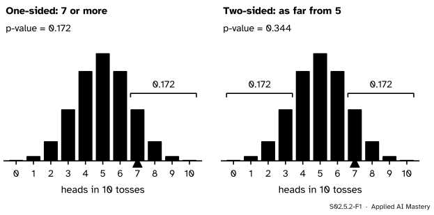
Seven heads in ten. One-sided, only a surplus of heads counts as extreme. Two-sided, a shortfall counts too: 3 or fewer is as far from 5 as 7 or more, so the p-value doubles.
If we only suspected a coin weighted towards heads, the extreme results are 7, 8, 9 and 10, and the p-value is 0.172. If any bias would interest us, 3 heads would have been just as striking as 7, so 0, 1, 2 and 3 join the tail and the p-value is \({2 \times 0.172 = 0.344}\).
Build it up
Step 1. The definition. The p-value is the probability, computed as if \(H_0\) were true, of a test statistic at least as extreme as the one observed. “Extreme” means “pointing towards \(H_1\)”.
Step 2. Two-sided for a count. For a symmetric null distribution, the two tails are mirror images, and the two-sided p-value is twice the one-sided one. When the null distribution is not symmetric, such as \({\mathrm{Bin}(100, 0.85)}\), there is no mirror. The rule scipy.stats.binomtest uses is to add the chances of every count no more likely than the observed one. For a fair coin the two rules agree.
Step 3. A statistic on a continuous scale. The city of S01 (invented) has a mean rent of \({\mu = 8.3}\) hundred euros a month with standard deviation \({\sigma = 5.41}\), known from its full register. A listing site says its flats are typical of the city. Twenty-five of its flats, drawn at random, have a mean rent of \({\bar{x} = 10.5}\). Is the site typical?
Take \({H_0 : \mu = 8.3}\) for the site’s flats, with the city’s spread. Under \(H_0\) the sample mean has standard error \({\sigma/\sqrt{n} = 5.41/5 = 1.082}\) (S02.1.2), and by the central limit theorem its distribution is close to normal. Standardise:
Step 4. The tail of a bell. Under \(H_0\), \(z\) follows \({N(0, 1)}\), whose distribution function is \({\Phi}\). Python has no \(\Phi\) in math, but it has the error function, and \({\Phi(z)}\)\({= \tfrac12\,(1 + \operatorname{erf}(z/\sqrt{2}))}\).
S02.5.2-F2
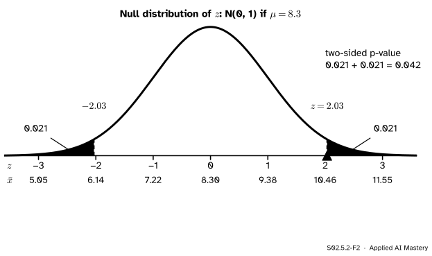
The z-test on its two scales. The observed mean 10.5 sits 2.03 standard errors above 8.3. Each yellow tail has area 0.021; one-sided the p-value is 0.021, two-sided 0.042.
A one-sided question (“is the site dearer?”) gives \({1 - \Phi(2.03) = 0.021}\). A two-sided one (“is the site different?”) gives twice that, 0.042.
The formal statement
NoteDefinition: the p-value
For a test statistic \(T\) whose large values point towards \(H_1\), and an observed value \(t\),
\[
\text{p-value} = \Prob(T \ge t \mid H_0).
\]
For the z-test with \({z = (\bar{x} - \mu_0)/(\sigma/\sqrt{n})}\):
The two-sided formula is the one-sided one applied to the statistic \({\abs{Z}}\): a value is at least as extreme as \(z\) when it lies at least as far from 0, on either side, and by symmetry \({\Prob(\abs{Z} \ge \abs{z})}\)\({= 2\,\Prob(Z \ge \abs{z})}\).
Under \(H_0\) the p-value is uniform. Treat the p-value as what it is before the data arrive: a random variable \({P = 1 - F(T)}\), where \(F\) is the distribution function of \(T\) under \(H_0\).
NoteTheorem
If \(T\) has a continuous, strictly increasing distribution function \(F\) under \(H_0\), then \({P = 1 - F(T)}\) satisfies \({\Prob(P \le u \mid H_0) = u}\) for every \(u\) in \({[0, 1]}\): the p-value is uniform on \({[0, 1]}\).
Proof. Fix \(u\) strictly between 0 and 1. Because \(F\) is continuous and climbs from 0 to 1, there is a cut-off \(t_u\) with \({1 - F(t_u) = u}\). Then each line below is the same event:
\[
\begin{aligned}
P \le u
&\iff 1 - F(T) \le u \\
&\iff F(T) \ge 1 - u = F(t_u) \\
&\iff T \ge t_u .
\end{aligned}
\]
The last step uses that \(F\) is strictly increasing, so it keeps the order of its inputs. Hence \({\Prob(P \le u)}\)\({= \Prob(T \ge t_u)}\)\({= 1 - F(t_u)}\)\({= u}\). For \({u = 0}\) and \({u = 1}\) the statement holds at the ends, since \(P\) lies between 0 and 1 and equals 0 with chance 0. ∎
S02.5.2-F3
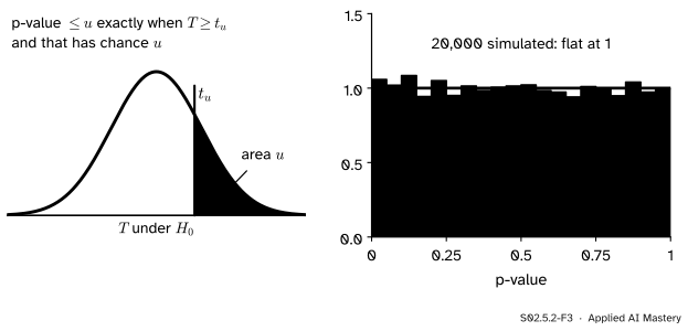
Left: the p-value is at most \(u\) exactly when \(T\) lands in the yellow tail, which has area \(u\). Right: p-values of 20,000 z-tests on data where \(H_0\) is true come out flat.
So when nothing is going on, a p-value below 0.05 turns up 5 percent of the time, one below 0.01 turns up 1 percent of the time, and every stretch of \({[0, 1]}\) of the same width is equally likely. This is what makes “reject when the p-value is below 0.05” a rule with a known false alarm rate, the subject of the next lesson.
Go deeper: a count is not continuous: the p-value is then 'at most uniform'
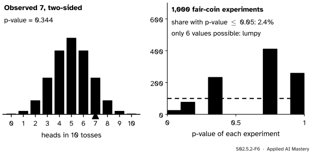
For the coin, \(T\) takes only 11 values, so the p-value takes only a few values too, and the theorem cannot hold exactly. What survives is an inequality: \({\Prob(P \le u) \le u}\) for every \(u\).
Write \({g(t) = \Prob(T \ge t \mid H_0)}\), the p-value of an observed \(t\); it can only fall as \(t\) grows. Given \(u\), let \(t^*\) be the smallest possible value of \(T\) with \({g(t^*) \le u}\). A value \(t\) has \({g(t) \le u}\) exactly when \({t \ge t^*}\), so
The same argument works for the two-sided rule, with “at least as extreme” meaning “no more likely”. For 10 tosses the two-sided p-values are 0.002, 0.021, 0.109, 0.344, 0.754 and 1, and \({\Prob(P \le 0.05) = 0.021}\), well under 0.05. A test on a count is conservative: it raises false alarms less often than its nominal rate. The interactive below shows the lumps, and how they shrink as the number of tosses grows.
Worked example
Are the listing site’s flats typical of the city?
S02.5.2-F4
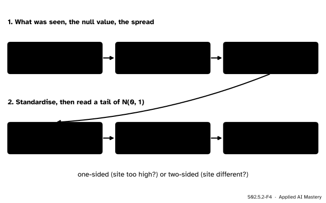
The z-test, traced. Everything after the first row is arithmetic and one lookup of \(\Phi\).
Ingredients. Data: \({n = 25}\) flats with \({\bar{x} = 10.5}\). Null: \({H_0 : \mu = 8.3}\), with \({\sigma = 5.41}\) known. The site claims to be typical, and a cheaper or a dearer site would both contradict it, so the alternative is two-sided, \({H_1 : \mu \neq 8.3}\).
Standard error.\({\sigma/\sqrt{n}}\)\({= 5.41/\sqrt{25}}\)\({= 5.41/5}\)\({= 1.082}\).
Tail.\({\Phi(2.033) = 0.979}\), so \({1 - \Phi(2.033) = 0.021}\), and the two-sided p-value is \({2 \times 0.021 = 0.042}\).
Read it. If the site’s flats were like the city’s, a sample mean at least this far from 8.3, in either direction, would turn up in about 4 samples of 25 out of 100. That is unusual enough to doubt the site’s claim. The next lesson turns “unusual enough” into a rule fixed in advance.
A caveat. City rents are skewed to the right, so the bell for \(\bar{x}\) at \({n = 25}\) is a good approximation, not exact (S02.1.3). The 0.042 is accurate to about the second decimal place.
Code
From scratch: \(\Phi\) from math.erf, then the two p-values of the worked example.
import mathdef Phi(z):"""The standard normal distribution function, from the error function."""return0.5* (1+ math.erf(z / math.sqrt(2)))mu0, sigma, n, xbar =8.3, 5.41, 25, 10.5se = sigma / math.sqrt(n)z = (xbar - mu0) / seone_sided =1- Phi(z)two_sided =2* (1- Phi(abs(z)))print(f"SE = {se:.3f}, z = {z:.3f}")print(f"one-sided p-value {one_sided:.4f}, two-sided {two_sided:.4f}")coin_one =sum(math.comb(10, k) for k inrange(7, 11)) /2**10print(f"coin: one-sided {coin_one:.3f}, two-sided {2* coin_one:.3f}")
SE = 1.082, z = 2.033
one-sided p-value 0.0210, two-sided 0.0420
coin: one-sided 0.172, two-sided 0.344
Now the theorem, checked by simulation: 20,000 samples of 25 drawn from a normal population where \(H_0\) is true, each turned into a two-sided p-value. The share in each tenth of \({[0, 1]}\) should be close to 0.1.
import numpy as nprng = np.random.default_rng(1)samples = rng.normal(mu0, sigma, size=(20_000, n))zs = (samples.mean(axis=1) - mu0) / sepvals = np.array([2* (1- Phi(abs(v))) for v in zs])shares = np.histogram(pvals, bins=10, range=(0, 1))[0] /len(pvals)print("share in each tenth:", np.round(shares, 3))print(f"share at or below 0.05: {np.mean(pvals <=0.05):.4f}")
share in each tenth: [0.103 0.099 0.098 0.097 0.103 0.096 0.101 0.102 0.101 0.101]
share at or below 0.05: 0.0514
Every tenth holds close to a tenth of the p-values, and close to 5 percent fall at or below 0.05, as the theorem promises. (The exact shares depend on the random draws; the checks allow for that.)
Finally the library. scipy.stats.norm.sf is the upper tail \({1 - \Phi}\), computed accurately even far out in the tail, and binomtest gives the coin’s two-sided p-value directly.
from scipy import statsprint(f"z-test: one-sided {stats.norm.sf(z):.4f}, two-sided {2* stats.norm.sf(abs(z)):.4f}")coin = stats.binomtest(7, n=10, p=0.5) # two-sided is the defaultprint(f"coin, two-sided: {coin.pvalue:.4f}")# the exact two-sided p-values for 10 tosses, and the chance of one at or below 0.05ps = [stats.binomtest(k, 10, 0.5).pvalue for k inrange(11)]pmf = stats.binom.pmf(range(11), 10, 0.5)print("distinct p-values:", sorted({round(p, 3) for p in ps}))print(f"P(p-value <= 0.05) = {sum(m for m, p inzip(pmf, ps) if p <=0.05):.4f}")
Set the number of tosses and the observed count, and choose one- or two-sided: the bars at least as extreme fill in and the read-out gives the p-value. Then run a thousand experiments in which the coin really is fair and watch their p-values stack up. Raise the number of tosses to see the lumps shrink, first near 0, or switch to the z-test, whose statistic is continuous, to see a flat histogram.
Notice that in coin mode the exact chance of a p-value at or below 0.05, shown in brackets in the read-out, never goes above 5 percent, while in z-test mode it is exactly 5 percent. The simulated share wanders a little around that exact chance from one batch of runs to the next. That is the theorem and the deeper block above, made visible.
Pitfalls
S02.5.2-F5
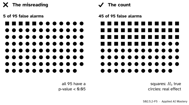
Wrong beside right, for 1,000 tests of which 900 have a true \(H_0\) and 100 a real effect that reaches a p-value below 0.05 half the time. Of the 95 “significant” results, 45 are false alarms: 47 percent, not 5 percent.
“The p-value is 0.03, so there is a 3 percent chance that \(H_0\) is true.”
The p-value is computed by assuming\(H_0\). It is \({\Prob(\text{data this extreme} \mid H_0)}\), not \({\Prob(H_0 \mid \text{data})}\). The two can be far apart. Suppose a team runs 1,000 tests: 900 changes do nothing and 100 have a real effect that reaches a p-value below 0.05 half the time. The 900 true nulls give about \({900 \times 0.05 = 45}\) false alarms and the real effects give 50 hits, so 45 of the 95 significant results, 47 percent, are false alarms. The chance that \(H_0\) is true given a significant result depends on how many true nulls there were to begin with, which the p-value knows nothing about; S04 makes that calculation with Bayes’ rule.
“A tiny p-value means a big effect.”
The p-value mixes the size of the effect with the amount of data. The same small gap from \(\mu_0\) gives a large p-value with a sample of 25 and a tiny one with a sample of 25,000, because the standard error shrinks like \({1/\sqrt{n}}\). Lesson S02.5.4 works an example, and S02.6 reports effects in their own right.
“The p-value is the probability that the result is due to chance alone.”
This sounds like a paraphrase of the definition, but it is the first misreading in disguise: “due to chance alone” is \(H_0\), so it again asks for \({\Prob(H_0 \mid \text{data})}\). The p-value assumes chance alone and asks how unusual the data would be.
Check yourself
Recall
1. Define the p-value in one sentence.
Show answer
The probability, computed as if \(H_0\) were true, of a test statistic at least as extreme (in the direction of \(H_1\)) as the one observed.
2. For 7 heads in 10 tosses, what are the one-sided and two-sided p-values, and why does one double the other?
Show answer
0.172 and 0.344. The null distribution \({\mathrm{Bin}(10, 0.5)}\) is symmetric about 5, so the tail at 3 or fewer is the mirror image of the tail at 7 or more.
3. How do you get \(\Phi(z)\) in plain Python?
Show answer
\({\Phi(z)}\)\({= \tfrac12\,(1 + \operatorname{erf}(z/\sqrt{2}))}\), with math.erf.
4. What is the distribution of a continuous test’s p-value when \(H_0\) is true?
Show answer
Uniform on \({[0, 1]}\): \({\Prob(P \le u) = u}\) for every \(u\). For a count it is conservative, \({\Prob(P \le u) \le u}\).
5. Why is a p-value of 0.03 not a 3 percent chance that \(H_0\) is true?
Show answer
It is computed assuming \(H_0\), so it is the chance of such data given \(H_0\). The chance of \(H_0\) given the data also depends on how often \(H_0\) is true in the first place.
Exercises
1.★ A second listing site’s 25 flats have mean rent 7.0. With \({\mu_0 = 8.3}\) and \({\sigma = 5.41}\), find \(z\) and the two-sided p-value.
Show solution
\({z = (7.0 - 8.3)/1.082 = -1.20}\). Two-sided, \({2\,(1 - \Phi(1.20))}\)\({= 2 \times 0.1148}\)\({= 0.230}\). A sample mean this far from 8.3 is common under \(H_0\); the data give no reason to doubt it. In code: 2 * stats.norm.sf(1.3 / 1.082) gives 0.230.
2.★★ A classifier gets 90 of 100 right and the baseline is 0.85. The one-sided p-value is 0.099. Explain why doubling it does not give the two-sided p-value, and say what stats.binomtest(90, 100, 0.85) computes instead.
Show solution
\({\mathrm{Bin}(100, 0.85)}\) is not symmetric about 85: its left tail is longer than its right, so there is no mirror image of “90 or more”. binomtest adds the chances of every count whose own chance is no larger than that of 90, that is, 90 and above together with the counts far enough below 85 to be as unlikely as 90 (80 and below). The result, about 0.21, is close to but not exactly \({2 \times 0.099}\).
3.★★★ Show that the two-sided z-test p-value \({P = 2\,(1 - \Phi(\abs{Z}))}\) is uniform on \({[0, 1]}\) when \({Z \sim N(0, 1)}\), by applying the theorem to \({T = \abs{Z}}\).
Show solution
For \({t \ge 0}\), \({G(t)}\)\({= \Prob(\abs{Z} \le t)}\)\({= \Phi(t) - \Phi(-t)}\)\({= 2\Phi(t) - 1}\), which is continuous and strictly increasing on \({[0, \infty)}\) and climbs from 0 to 1. Since \({\abs{Z}}\) only takes values in \({[0, \infty)}\), every step of the proof goes through. So \({1 - G(\abs{Z})}\)\({= 2 - 2\Phi(\abs{Z})}\)\({= 2\,(1 - \Phi(\abs{Z}))}\)\({= P}\). The theorem, applied to \({T = \abs{Z}}\) with distribution function \(G\), gives \({\Prob(P \le u) = u}\) for every \(u\) in \({[0, 1]}\).
Summary card
The p-value is the chance under \(H_0\) of a result at least as extreme as the one seen.
Under \(H_0\). Uniform on \({[0, 1]}\) for a continuous statistic; at most uniform for a count.
Not the probability that \(H_0\) is true, and not the size of the effect.
Sources and next steps
Sources. Each was opened and checked against this lesson on 15 November 2026.
Jeremy Orloff and Jonathan Bloom, Reading 17b, Null Hypothesis Significance Testing I, MIT OpenCourseWare 18.05 (Spring 2022). Section 7 defines the p-value as the probability, assuming the null hypothesis, of data at least as extreme as the experimental data, and Section 7.1 works a one-sided z-test (Example 13) by standardising the sample mean.
David Diez, Mine Cetinkaya-Rundel and Christopher Barr, OpenIntro Statistics, fourth edition (free PDF). Section 5.3.4, formal testing using p-values: the p-value as the probability of data at least as favourable to the alternative as the current data, if the null hypothesis were true.
American Statistical Association, press release on its Statement on Statistical Significance and P-Values, 7 March 2016. It lists the statement’s six principles; the second says that p-values do not measure the probability that the studied hypothesis is true, or the probability that the data were produced by random chance alone, and the fifth that a p-value does not measure the size of an effect.