Test twenty true null hypotheses at level 0.05 and the chance of at least one false positive is 0.64. Derive that number, define the family-wise error rate, and see the same trap in the garden of forking paths and in picking the best of many models or features.
S02.9.1L2 Intermediate25 minIn review (what this means)
The maths and code on this page are checked by automated tests on every change, but an independent reader has not signed it off yet. Spot a mistake or a confusing step? Tell us.
Derive the chance of at least one false positive among m independent tests of true nulls, 1 − (1 − α)^m, and evaluate it for 20 tests at level 0.05.
Define a family of tests and its family-wise error rate, and show that the expected number of false positives is m₀α whether or not the tests are independent.
Explain the garden of forking paths: analyses that were never run, but would have been on other data, count as tests.
Recognise picking the best of many features or models on one validation set as a multiple-testing problem.
The question
You screen 20 features for a link with whether customers leave, testing each at level 0.05. In truth none of them has any link at all. How likely is it that at least one comes out “significant” anyway, and what does that do to a model built on the features that survive?
Intuition
One test at level 0.05 promises something modest: if its null hypothesis is true, it cries wolf 5 percent of the time. Run twenty such tests and each one keeps that promise, yet the twenty together break it. Every test is a fresh chance for a false alarm, and the chances pile up.
S02.9.1-F1
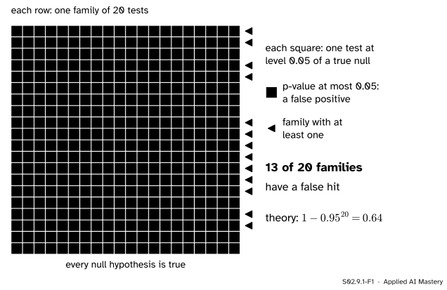
Twenty simulated families of 20 tests in which every null is true (seed 1). Each test alone errs 5 percent of the time, but 13 of the 20 families contain at least one false positive, close to the 64 percent that theory gives.
Look along any single column: about one square in twenty is purple, exactly as promised. Now look along a row. A row is what one analyst sees: a whole screen of 20 features. Most rows hold a purple square somewhere. The analyst who reports “feature 7 is significant” is reporting the row’s luckiest square, and luck is what put it there.
Build it up
Step 1. One test. If the null is true and the test has level \(\alpha = 0.05\), the chance of a false positive is 0.05, so the chance of none is \({1 - 0.05} = 0.95\).
Step 2. Two independent tests. Both must stay quiet. Independent events multiply, so the chance of no false positive is \({0.95 \times 0.95} = 0.9025\), and the chance of at least one is \({1 - 0.9025} = 0.0975\): nearly double.
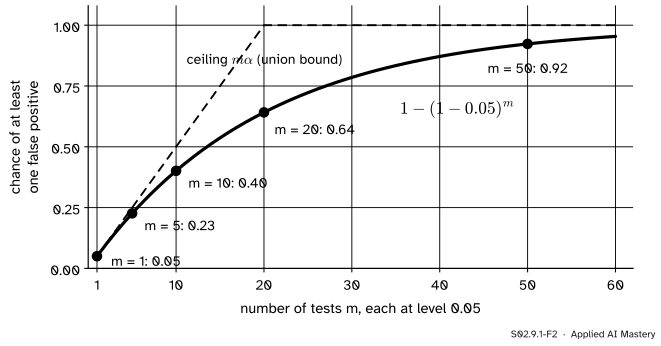
Step 3. Any number. With \(m\) independent tests the chance of no false positive is \({0.95^m}\), and of at least one is \({1 - 0.95^m}\). It is 0.23 for 5 tests, 0.40 for 10, 0.64 for 20 and 0.92 for 50.
S02.9.1-F2
The chance of at least one false positive among \(m\) independent tests of true nulls at level 0.05. The dashed ceiling \(m\alpha\) holds for any tests, independent or not (lesson S02.9.2).
Step 4. Count the false positives instead. Each test of a true null is a coin that lands “false positive” with chance 0.05. Twenty of them give, on average, \({20 \times 0.05} = 1\) false positive. One per screen is the typical result of testing pure noise.
The formal statement
A family is a set of \(m\) hypotheses \(H_1, \dots, H_m\) that are tested together and whose results are read together. Of these, \(m_0\) are true nulls. Let \(V\) be the number of true nulls that are rejected, the false positives (or false discoveries).
NoteDefinition: family-wise error rate
The family-wise error rate is the chance of at least one false positive in the family:
\[
\text{FWER} = \Prob(V \geq 1).
\]
If the \(m_0\) true nulls are tested independently, each with a false-positive chance of exactly \(\alpha\) (a level-\(\alpha\) test on a continuous statistic),
The second result holds whether or not the tests are independent.
Derivation of the FWER. Let \(A_i\) be the event “test \(i\) rejects”, for each true null \(i\). A valid test of a true null has \({\Prob(A_i) \leq \alpha}\), with equality for a continuous statistic, since the p-value is then uniform (S02.5.2). The complement of “at least one rejects” is “none rejects”, the intersection of the complements:
Derivation of \(\E[V]\). Write \(V\) as a sum of indicators, \({V = \sum_i I_i}\), where \(I_i\) is 1 when test \(i\) rejects and 0 otherwise. The expectation of a sum is the sum of the expectations, independent or not, and the expectation of an indicator is the probability of its event:
Two extremes. If the 20 tests were the same test copied 20 times, they would all reject or all stay quiet together, and the FWER would be 0.05. If they are independent, it is 0.64. Real families sit between: tests that share data are often positively related, and then their FWER is somewhat lower than the independent value, but it is still far above 0.05. The next lesson proves that \({\text{FWER} \leq m_0\alpha}\) always, the dashed ceiling of the build-up figure.
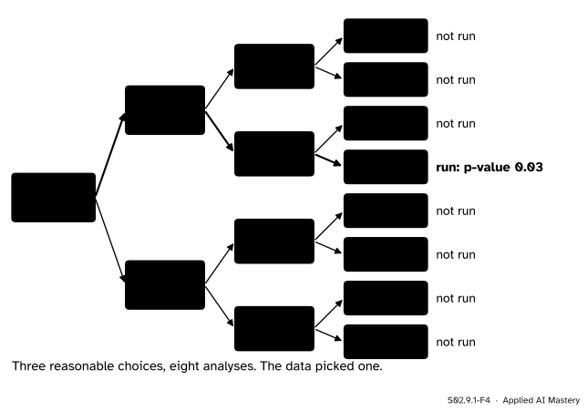
The tests you could have run. A family need not be written down. Gelman and Loken call it the garden of forking paths: an analysis has many reasonable choices (which outliers to drop, which outcome to measure, which users to include), and the data themselves nudge the analyst down one path. Only one test is run, yet the false-positive rate is that of the whole garden, because other data would have led to another path and another test.
S02.9.1-F4
The garden of forking paths. Three yes-or-no choices give eight analyses. One was run, but the data chose which, so all eight belong to the family.
Where machine learning meets it. Screening features one test at a time is a family. So is choosing the best of many models on one validation set: each comparison with a baseline is a test, and the winner’s validation score is the largest of many noisy scores (ML01.9.4).
Worked example
Twenty noise features at level 0.05. Here \(m = m_0 = 20\) and \(\alpha = 0.05\), and the features are independent.
S02.9.1-F3
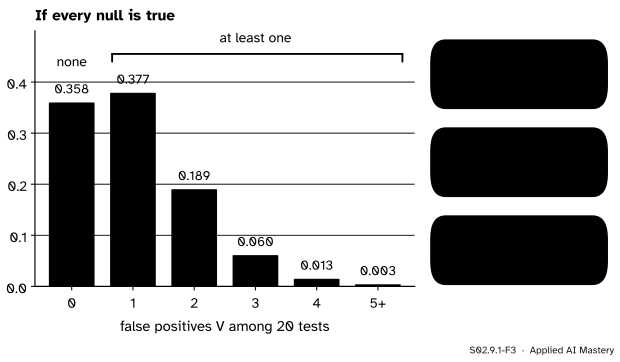
The number of false positives among 20 independent true-null tests is binomial, \({\text{Bin}(20, 0.05)}\). No false positive is less likely than exactly one.
No false positive: \({0.95^{20}} = 0.358\). Square 0.95 four times over to check by hand: \({0.95^2} = 0.9025\), \({0.95^4} = 0.8145\), \({0.95^8} = 0.6634\), \({0.95^{16}} = 0.4401\), and \({0.95^{20}} = {0.4401 \times 0.8145} = 0.358\).
At least one: \({1 - 0.358} = 0.642\), the 0.64 of the hook.
Expected number: \({20 \times 0.05} = 1\).
Exactly one: \({20 \times 0.05 \times 0.95^{19}} = 0.377\), which is larger than the chance of none.
So a screen of 20 pure-noise features usually “finds” something, and the most likely outcome is one spurious feature.
Code
From the formula, then by simulation: 10,000 families of 20 true-null p-values, each uniform on \([0, 1]\).
import numpy as npfrom scipy import statsalpha, m =0.05, 20fwer =1- (1- alpha) ** mprint(f"formula: FWER = {fwer:.4f}, expected false positives = {m * alpha:.2f}")print("for m = 1, 5, 10, 50:", [round(1- (1- alpha) ** k, 3) for k in (1, 5, 10, 50)])rng = np.random.default_rng(1)p = rng.uniform(size=(10_000, m)) # every null true: p-values are uniformhits = (p <= alpha).sum(axis=1) # V for each familyprint(f"simulated: FWER = {np.mean(hits >=1):.4f}, mean V = {hits.mean():.3f}")print("Bin(20, 0.05) at 0, 1, 2:", np.round(stats.binom.pmf([0, 1, 2], m, alpha), 3))
formula: FWER = 0.6415, expected false positives = 1.00
for m = 1, 5, 10, 50: [0.05, 0.226, 0.401, 0.923]
simulated: FWER = 0.6413, mean V = 0.996
Bin(20, 0.05) at 0, 1, 2: [0.358 0.377 0.189]
Now the hook itself: 20 features of pure noise, each tested for correlation with a target over 100 rows, 2,000 times over. The test is the usual t-test of a correlation, \(r\) turned into \({t = r\sqrt{(n - 2)/(1 - r^2)}}\) on \({n - 2}\) degrees of freedom; scipy.stats.pearsonr gives the same p-value.
rng = np.random.default_rng(7)n, d, reps =100, 20, 2000found =0for _ inrange(reps): X = rng.normal(size=(n, d)) # 20 features of noise y = rng.normal(size=n) # a target unrelated to all of them Xc, yc = X - X.mean(0), y - y.mean() r = (Xc * yc[:, None]).sum(0) / np.sqrt((Xc **2).sum(0) * (yc **2).sum()) t = r * np.sqrt((n -2) / (1- r **2)) pv =2* stats.t.sf(np.abs(t), n -2) found += np.any(pv <= alpha)print(f"screens with at least one 'significant' noise feature: {found / reps:.3f}")print("check one feature with scipy:", stats.pearsonr(X[:, 0], y).pvalue, pv[0])
screens with at least one 'significant' noise feature: 0.644
check one feature with scipy: 0.009883617091196839 0.009883617091196794
About 64 percent of screens, as the formula said: correlation tests on separate noise features are independent enough for the product rule to hold.
Explore
This module’s interactive, the many-tests simulator, is in lesson S02.9.3. To see this lesson in it, set the share of real effects to 0 and the number of tests to 20, then press New p-values again and again: the uncorrected cut at 0.05 catches at least one point in roughly two presses out of three.
Pitfalls
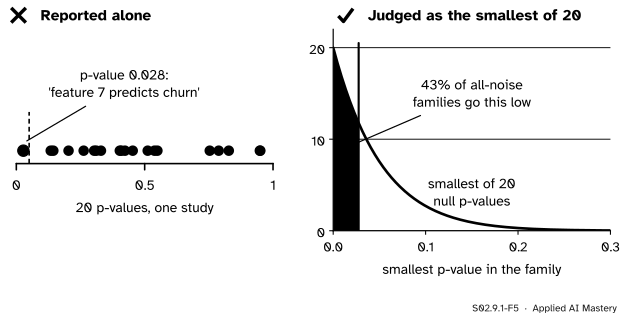
S02.9.1-F5
Wrong beside right. Read alone, 0.028 looks like a finding. Read as what it is, the smallest of 20 p-values, it is unremarkable: 43 percent of families of pure noise produce a minimum this small.
“Each test was at level 0.05, so my error rate is 0.05.”
The level is a promise about one test. The reader of a screen cares about the family: did any reported finding come from noise? For 20 independent tests of true nulls that happens 64 percent of the time. Say which error rate you control, and control the family’s (S02.9.2).
“I only ran one analysis, so there is nothing to correct.”
If the choice of analysis followed the data, the family is every analysis the data could have led you to. Gelman and Loken’s point is that no fishing is needed: a reasonable analyst, reacting honestly to the data, still walks the garden. Fix the analysis before seeing the data, or treat it as exploratory.
“The tests are correlated, so the problem goes away.”
Positive dependence lowers the FWER below \({1 - (1 - \alpha)^m}\), but only perfect dependence brings it down to \(\alpha\). And the expected number of false positives, \({m_0 \alpha}\), does not depend on dependence at all.
Check yourself
Recall
1. What is the family-wise error rate?
Show answer
The probability of at least one false positive among all the tests of a family, \({\Prob(V \geq 1)}\).
2. What is the FWER of 20 independent tests of true nulls, each at level 0.05?
Show answer
\({1 - 0.95^{20}} = 0.64\).
3. How many false positives do 20 tests of true nulls at level 0.05 give on average, and does the answer need independence?
Show answer
\({20 \times 0.05} = 1\). No: the expectation of a sum of indicators is the sum of their probabilities whatever the dependence.
4. What is the garden of forking paths?
Show answer
The many analyses that reasonable choices could have produced. When the data steer which one is run, the false-positive rate is that of the whole set of possible analyses, even though only one test was carried out.
5. Why is choosing the best of many models on one validation set a multiple-testing problem?
Show answer
Each candidate is a test against the baseline, and the winner’s score is the largest of many noisy scores, so it looks better than it is even when no candidate is truly better.
Exercises
1.★ Ten independent tests of true nulls are run at level 0.01. Find the FWER and the expected number of false positives.
Show solution
FWER \({= 1 - 0.99^{10}} = {1 - 0.9044} = 0.0956\). Expected number \({10 \times 0.01} = 0.1\). A stricter level per test is what keeps the family’s rate below 0.1: lesson S02.9.2 turns this into a rule.
2.★★ How many independent tests of true nulls at level 0.05 does it take before a false positive somewhere is more likely than not?
Show solution
We need \({1 - 0.95^m} > 0.5\), that is \({0.95^m} < 0.5\). Take logarithms; \({\ln 0.95}\) is negative, so dividing by it flips the inequality:
So 14 tests: \({1 - 0.95^{14}} = 0.512\), while 13 give \({1 - 0.95^{13}} = 0.487\).
3.★★★ Prove that \({1 - (1 - \alpha)^m} \leq m\alpha\) for every whole number \(m \geq 1\) and every \(\alpha\) in \([0, 1]\), so the independent FWER always sits under the ceiling \(m\alpha\).
Show solution
Equivalently, show \({(1 - \alpha)^m} \geq {1 - m\alpha}\) by induction on \(m\). For \(m = 1\) both sides equal \({1 - \alpha}\). Suppose it holds for \(m\). If \({1 - m\alpha} < 0\) the claim for \({m + 1}\) is immediate, since the left side is at least 0 and the right side is smaller still. Otherwise multiply both sides by \({1 - \alpha} \geq 0\):
because \({m\alpha^2} \geq 0\). This is Bernoulli’s inequality. For 20 tests at 0.05 the ceiling is 1, so it says little; for 5 tests it gives 0.25 against the true 0.226.
Summary card
Every test is a fresh chance for a false alarm, and the chances pile up.
Independent tests.\({\text{FWER} = 1 - (1 - \alpha)^{m_0}}\): 0.64 for 20 at 0.05.
Any tests.\({\E[V] = m_0\alpha}\), and \({\text{FWER} \leq m_0\alpha}\).
Forking paths. Analyses the data could have chosen count as tests.
Sources and next steps
Sources. Each was opened and checked against this lesson on 15 November 2026.
Siva Balakrishnan, Lecture 23, 36-705 Intermediate Statistics, Carnegie Mellon University, Fall 2019. Section 23.2 sets out the multiple-testing problem (1,000 tests at 0.05 give about 50 false rejections) and Section 23.2.1 defines the family-wise error rate as the probability of falsely rejecting even once among the tests.
Andrew Gelman and Eric Loken, The garden of forking paths, 14 November 2013. The abstract and Sections 1.1 and 1.2 argue that multiple comparisons arise even when only one analysis is run, because the analysis is contingent on the data.