When many hypotheses are tested and some real effects are expected, control the average share of false discoveries instead of the chance of any. Derive the Benjamini-Hochberg sloped line, run it by hand on ten p-values, prove its guarantee and check it with scipy.stats.false_discovery_control.
S02.9.3L2 Intermediate25 minIn review (what this means)
The maths and code on this page are checked by automated tests on every change, but an independent reader has not signed it off yet. Spot a mistake or a confusing step? Tell us.
Define the false discovery proportion and the false discovery rate, and explain how the rate differs from the family-wise error rate.
Carry out the Benjamini-Hochberg procedure by hand, rejecting the k smallest p-values for the largest k with p₍ₖ₎ ≤ kq/m.
State the guarantee FDR ≤ q m₀/m for independent tests, check it by simulation, and name Benjamini-Yekutieli for arbitrary dependence.
Compute Benjamini-Hochberg adjusted p-values from scratch and with scipy.stats.false_discovery_control.
The question
You screen 100 features, and, unknown to you, 20 of them carry a real signal. Bonferroni at 0.05 finds about 8 of the 20 and almost never a false one. Would you accept a few false finds in exchange for many more real ones, if on average no more than 5 percent of what you report were false? That trade has a name, and a procedure that makes it.
From the last lesson
1. In Holm’s procedure, what is the \(k\)-th smallest p-value compared with?
Show answer
With \({\alpha/(m - k + 1)}\), and the procedure stops at the first p-value that misses its step.
2. Does Bonferroni’s guarantee need the tests to be independent?
Show answer
No. The union bound needs nothing about dependence.
Intuition
The family-wise error rate asks for no false discovery at all, and pays for it with power. In a screen of thousands of genes, features or metrics, a few false leads among many real ones are a cost you can carry, so long as you know their share. The false discovery rate controls that share, on average.
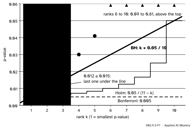
The rule that does it, from Benjamini and Hochberg, replaces the flat line and the steps with a straight line through the origin: the \(k\)-th smallest p-value may be up to \({k q/m}\).
S02.9.3-F1
The ten p-values under three cut-offs at level 0.05. The Benjamini-Hochberg line rises with the rank, so it rejects three where Bonferroni and Holm reject one.
The line is generous to the third p-value, 0.012, because by then two discoveries have already been made: one more false lead among three would still be a small share.
Build it up
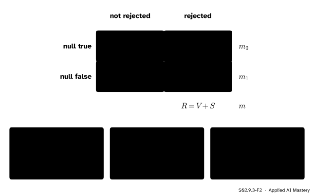
Step 1. Name the outcomes. Of \(m\) hypotheses, \(m_0\) are true nulls and \(m_1\) are false. A procedure rejects \(R\) of them; \(V\) of those are false discoveries and \(S\) are true ones.
S02.9.3-F2
The four outcomes of \(m\) tests, after Benjamini and Hochberg. The FWER looks only at whether \(V \geq 1\); the FDR looks at \(V\) as a share of \(R\).
Step 2. A share, not a count. The false discovery proportion is \({V/R}\), the share of discoveries that are false, set to 0 when there are none. It is known only to someone who knows the truth. Its average over repetitions of the study is the false discovery rate.
Step 3. Where the line comes from. Suppose we reject every p-value up to a cut-off \(u\). Each true null has \({\Prob(\text{p}_i \leq u) = u}\), so about \({m_0 u}\) of the rejections are false, and \({m_0 u \leq m u}\). If the cut-off sits at the \(k\)-th smallest p-value, there are \(k\) rejections, and the estimated share of false ones is
Asking for this share to be at most \(q\) gives \({\text{p}_{(k)} \leq k q/m}\): the sloped line.
Step 4. Go as far as the line allows. Take the largest\(k\) that meets the condition, and reject the \(k\) smallest p-values. A p-value above the line at a lower rank is still rejected if a later one dips under. This is a step-up procedure; Holm’s was step-down.
The formal statement
NoteDefinition: the false discovery rate and the BH procedure
and reject \({H_{(1)}, \dots, H_{(k)}}\) (none if no \(j\) qualifies). If the p-values of the true nulls are independent of each other and of the false nulls’ p-values,
\[
\text{FDR} \leq \frac{m_0}{m}\, q \leq q .
\]
The guarantee is proved below for continuous p-values, where it holds with equality. It also holds under a kind of positive dependence that Benjamini and Yekutieli called PRDS.
Go deeper: a proof of the guarantee, for independent continuous p-values
Write the FDP as a sum over the true nulls, \({\text{FDP} = \sum_{i \in I_0} D_i/\max(R, 1)}\), where \(D_i\) is 1 when \(H_i\) is rejected. BH rejects \(H_i\) exactly when \({\text{p}_i \leq R q/m}\).
Let \(R_i\) be the number of rejections BH would make if \(\text{p}_i\) were replaced by 0. It depends only on the other p-values, so it is independent of \(\text{p}_i\).
Claim: \(H_i\) is rejected exactly when \({\text{p}_i \leq R_i q/m}\), and then \({R = R_i}\). If \(H_i\) is rejected with \(R = r\), lowering \(\text{p}_i\) to 0 keeps it among the \(r\) smallest, does not raise the \(r\)-th smallest, and leaves every larger order statistic as it was, so there are still \(r\) rejections: \({R_i = r}\) and \({\text{p}_i \leq r q/m}\). Conversely, if \({\text{p}_i \leq R_i q/m}\), raising \(\text{p}_i\) from 0 back to its value leaves at least \(R_i\) p-values at most \({R_i q/m}\), so \({R \geq R_i}\); and raising one value cannot lower any order statistic, so no rank beyond \(R_i\) qualifies: \({R = R_i}\).
So \({D_i/\max(R, 1)}\) equals \({1/R_i}\) when \({\text{p}_i \leq R_i q/m}\) and 0 otherwise. Condition on \(R_i\); since \(\text{p}_i\) is uniform and independent of it,
Average over \(R_i\) and add over the \(m_0\) true nulls: \({\text{FDR} = m_0 q/m}\).
FDR and FWER. The FDP is at most 1, and it is 0 when \({V = 0}\), so \({\text{FDP} \leq 1}\) on the event \({V \geq 1}\) and 0 otherwise. Taking expectations, \({\text{FDR} \leq \Prob(V \geq 1)}\): the FDR is never above the FWER. If every null is true, any rejection is false, the FDP is 1 whenever \({V \geq 1}\), and the two are equal. So BH holds the FWER at \(q\) when there is nothing to find, and relaxes only when there is.
Adjusted p-values.\(H_{(k)}\) is rejected at level \(q\) when some \({j \geq k}\) has \({\text{p}_{(j)} \leq j q/m}\), that is when \({\min_{j \geq k} m\,\text{p}_{(j)}/j \leq q}\):
Any dependence: Benjamini-Yekutieli. Divide \(q\) by \({c(m) = 1 + \tfrac12 + \dots + \tfrac1m}\) and run BH. This controls the FDR at \(q\) for any dependence. For ten tests \({c(10) = 2.929}\), so the line becomes \({k \times 0.0171}/10\).
S02.9.3-F4
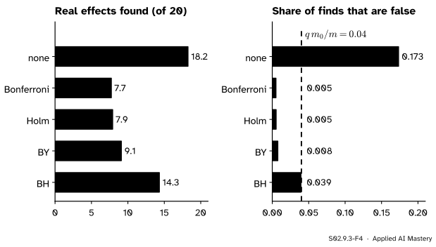
5,000 simulated screens of 100 tests, 20 with a real effect (seed 11). BH finds nearly twice as many real effects as Bonferroni, and its share of false finds sits on the promised \({q\,m_0/m}\).
Worked example
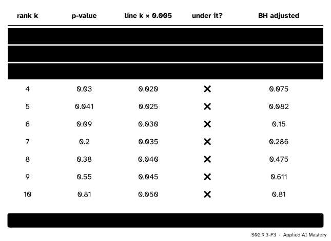
BH on the ten p-values at \({q = 0.05}\). The line is \({k \times 0.05/10} = {0.005\,k}\).
S02.9.3-F3
Benjamini-Hochberg, row by row. Unlike Holm, every row is checked; the decision rests on the last row under the line.
Compare each sorted p-value with its line value: \({0.001 \leq 0.005}\), \({0.008 \leq 0.010}\), \({0.012 \leq 0.015}\), but \({0.030 > 0.020}\), \({0.041 > 0.025}\), and every later one is above its line too.
The largest \(k\) under the line is 3, so BH rejects three, against one for Bonferroni and Holm.
Adjusted values, from the top down. Rank 10: \({10 \times 0.81/10} = 0.81\). Rank 9: \({10 \times 0.55/9} = 0.611\). Continuing gives 0.475, 0.286, 0.15, 0.082 and 0.075. Rank 3: \({10 \times 0.012/3} = 0.04\). Rank 2: \({10 \times 0.008/2} = 0.04\). Rank 1: \({10 \times 0.001/1} = 0.01\). Each is the minimum of its own ratio and the one above, and here the ratios already increase.
Benjamini-Yekutieli: \({0.05/2.929} = 0.0171\) replaces 0.05, so the line is \({0.00171\,k}\). Only 0.001 is under it: one rejection.
Code
From scratch, then the SciPy call.
import numpy as npfrom scipy import statspvals = np.array([0.001, 0.008, 0.012, 0.030, 0.041, 0.09, 0.20, 0.38, 0.55, 0.81]) # inventedq, m =0.05, len(pvals)def bh_adjusted(p): p = np.asarray(p) n =len(p) order = np.argsort(p) ratios = n * p[order] / np.arange(1, n +1) # m p_(k) / k adjusted = np.empty_like(p) adjusted[order] = np.minimum(1, np.minimum.accumulate(ratios[::-1])[::-1])return adjustedours = bh_adjusted(pvals)c10 =sum(1/ i for i inrange(1, m +1))print("BH adjusted:", ours.round(3), "rejects", int(np.sum(ours <= q)))print("scipy 'bh': ", stats.false_discovery_control(pvals).round(3))print("scipy 'by': ", stats.false_discovery_control(pvals, method="by").round(3),"rejects", int(np.sum(stats.false_discovery_control(pvals, method="by") <= q)), " c(10) =", round(c10, 3))
Benjamini-Yekutieli’s adjusted values are BH’s multiplied by \({c(10)}\) and capped at 1. Now the hook as a simulation: 5,000 screens of 100 one-sided z-tests, the first 20 with a real effect of 3 standard errors (seed 11).
rng = np.random.default_rng(11)z = rng.normal(size=(5000, 100))z[:, :20] +=3p = stats.norm.sf(z)def summary(rejected): v, r = rejected[:, 20:].sum(1), rejected.sum(1) fdp = np.where(r >0, v / np.maximum(r, 1), 0.0)return rejected[:, :20].sum(1).mean(), fdp.mean(), fdpbh = stats.false_discovery_control(p, axis=1) <= q # BH on each screenfound_bh, fdr_bh, fdp_bh = summary(bh)found_bon, fdr_bon, _ = summary(p <= q /100)print(f"BH: finds {found_bh:.1f} of 20, FDR {fdr_bh:.3f} (promised {q *80/100})")print(f"Bonferroni: finds {found_bon:.1f} of 20, FDR {fdr_bon:.3f}")print(f"BH studies with FDP 0: {np.mean(fdp_bh ==0):.2f}, with FDP above 0.1: {np.mean(fdp_bh >0.1):.2f}")fwer_bh = np.mean(bh[:, 20:].any(1))print(f"BH studies with at least one false find (its FWER): {fwer_bh:.3f}")
BH: finds 14.3 of 20, FDR 0.039 (promised 0.04)
Bonferroni: finds 7.7 of 20, FDR 0.005
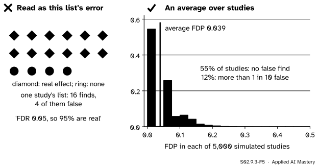
BH studies with FDP 0: 0.55, with FDP above 0.1: 0.12
BH studies with at least one false find (its FWER): 0.455
BH finds about 14.3 of the 20 real effects to Bonferroni’s 7.7, and its false discovery rate is 0.039, on the promised \({0.05 \times 80/100} = 0.04\).
Explore
S02.9-X1
Many-tests simulator
Set the number of tests, the share with a real effect, its size and the level, then press New p-values. Real effects are filled diamonds, true nulls hollow circles. The read-out counts each method’s rejections, false rejections and false discovery proportion; Average 500 runs estimates the rates.
Things to try. Press The ten p-values to see the worked example. Set the share of real effects to 0: the three methods then reject almost nothing, and averaged over 500 runs each one’s FWER is about the level. Set 100 tests, 20 percent real, effect 3: BH’s average FDP settles near \({0.05 \times 0.8} = 0.04\) while it finds nearly twice what Bonferroni finds. Raise the share of real effects to 80 percent: BH’s line now catches most of them, and its FDR falls to about \({0.05 \times 0.2} = 0.01\).
Pitfalls
S02.9.3-F5
Wrong beside right. The FDR is the average of the FDP over studies like yours. One list can be much worse than the average, as this one, with 4 of 16 finds false, is.
“FDR 0.05, so 95 percent of my discoveries are real.”
That is a statement about the average over repetitions. In the simulation, 12 percent of studies had more than one false find in ten. Report the FDR level you controlled, not a promise about this list.
“Like Holm, stop at the first p-value above the line.”
BH steps up: it takes the largest \(k\) under the line, even if an earlier p-value was above. Stopping early throws away discoveries that the guarantee already allows (exercise 2).
“BH controls the family-wise error rate.”
Only when every null is true. With real effects present, BH lets false discoveries in on purpose: in the simulation about 45 percent of studies had at least one. Use Holm when a single false claim is costly.
“My features are correlated, so BH is invalid.”
BH still controls the FDR under positive dependence of the PRDS kind, which covers many one-sided tests on positively correlated statistics. For arbitrary dependence, use method="by", at the cost of the factor \({c(m)}\).
Check yourself
Recall
1. Define the false discovery proportion and the false discovery rate.
Show answer
\({\text{FDP} = V/\max(R, 1)}\), the share of rejections that are false (0 if there are none); the FDR is its expectation.
2. State the Benjamini-Hochberg rule at level \(q\).
Show answer
Find the largest \(k\) with \({\text{p}_{(k)} \leq k q/m}\) and reject the \(k\) smallest p-values.
3. How many of the ten p-values does BH reject at \({q = 0.05}\), and how many do Bonferroni and Holm reject?
4. Why are the FDR and the FWER equal when every null is true?
Show answer
Then every rejection is false, so the FDP is 1 whenever \({V \geq 1}\) and 0 otherwise; its expectation is \({\Prob(V \geq 1)}\).
5. What does Benjamini-Yekutieli change, and why?
Show answer
It divides \(q\) by \({c(m) = \sum_{i=1}^m 1/i}\) (2.929 for ten tests), which makes the FDR at most \(q\) under any dependence between the tests.
Exercises
1.★ Five tests give p-values 0.008, 0.020, 0.024, 0.039 and 0.21. Apply BH, Holm and Bonferroni at level 0.05.
Show solution
The BH line is \({k \times 0.05/5} = {0.01\,k}\): 0.01, 0.02, 0.03, 0.04, 0.05. The first four p-values are under it and 0.21 is not, so BH rejects four. Bonferroni’s cut-off is 0.01: one rejection. Holm: \({0.008 \leq 0.01}\), reject; \({0.020 > 0.05/4} = 0.0125\), stop: one rejection.
2.★★ Four p-values, 0.004, 0.030, 0.034 and 0.80, at \({q = 0.05}\). Apply BH, and then the wrong rule that stops at the first p-value above the line. Compute the BH adjusted values.
Show solution
The line is \({0.0125\,k}\): 0.0125, 0.025, 0.0375, 0.05. Rank 1 passes, rank 2 (0.030) fails, rank 3 (\({0.034 \leq 0.0375}\)) passes, rank 4 fails. The largest passing \(k\) is 3, so BH rejects three, including 0.030. The wrong rule stops at rank 2 and rejects one.
The ratios \({4\,\text{p}_{(k)}/k}\) are 0.016, 0.06, 0.0453 and 0.8. Taking the minimum from the top down: \({\tilde{\text{p}}_{(4)} = 0.8}\), \({\tilde{\text{p}}_{(3)} = 0.0453}\), \({\tilde{\text{p}}_{(2)} = \min(0.06, 0.0453)} = 0.0453\), \({\tilde{\text{p}}_{(1)} = 0.016}\). Three are at most 0.05, as before.
3.★★★ Show that \({\text{FDR} \leq \text{FWER}}\) for any procedure, and that a procedure controlling the FWER at \(\alpha\) therefore controls the FDR at \(\alpha\).
Show solution
If \({V = 0}\), the FDP is 0. If \({V \geq 1}\), then \({R \geq V \geq 1}\) and the FDP is \({V/R}\), at most 1. So the FDP is never larger than the indicator of \({V \geq 1}\). Expectations keep inequalities, and the expectation of an indicator is the probability of its event:
If the FWER is at most \(\alpha\), so is the FDR. The converse fails: BH’s FWER in the simulation was about 0.45.
Summary card
Control the share of false finds, and the line may rise with the rank.
S02.9.3-F1
BH: 3. Holm and Bonferroni: 1.
FDR.\({\E[V/\max(R, 1)]}\), never above the FWER, equal to it when every null is true.
BH. Largest \(k\) with \({\text{p}_{(k)} \leq k q/m}\); reject the \(k\) smallest.
Guarantee.\({\text{FDR} \leq q\,m_0/m}\) for independent tests.
Any dependence. Benjamini-Yekutieli: \(q\) divided by \({c(m) = \sum_i 1/i}\).
Sources and next steps
Sources. Each was opened and checked against this lesson on 15 November 2026.
Siva Balakrishnan, Lecture 24, 36-705 Intermediate Statistics, Carnegie Mellon University, Fall 2019. Section 24.2 defines the FDP and the FDR, shows that the FDR equals the FWER under the global null and never exceeds it, and states the BH procedure with its sloped thresholds \({i\alpha/d}\), with a picture of the line crossing the sorted p-values.
Philip B. Stark, Ninth set of notes: Multiplicity, Statistics 210B, University of California, Berkeley. Section 3 follows the notation of Benjamini and Hochberg (1995), defines the procedure that rejects the hypotheses of the \({K(q^*)}\) smallest p-values, and states their Theorem 1, FDR control for independent test statistics, with their lemma giving the bound \({m_0 q^*/m}\).
SciPy developers, scipy.stats.false_discovery_control: methods 'bh' and 'by', the bound \({q\,m_0/m}\) for independent tests or tests with positive regression dependence, and the more conservative Benjamini-Yekutieli method for dependent ones, citing Benjamini and Hochberg (1995) and Benjamini and Yekutieli (2001).
Gilles Blanchard and Étienne Roquain, Two simple sufficient conditions for FDR control, Electronic Journal of Statistics 2 (2008). Section 3.1 presents BH as the linear step-up procedure and the procedure with the level divided by \({\sum_{i} 1/i}\) as the distribution-free one of Benjamini and Yekutieli; Section 3.2 covers the PRDS condition.
Next.S02.9.4 Multiplicity in practice takes these corrections to ANOVA comparisons, experiments with many metrics, feature screens and leaderboards.