Controlling the family-wise error: Bonferroni and Holm
Split the level alpha among m tests and the union bound keeps the chance of any false positive at most alpha, with no independence needed. Prove it for Bonferroni and for Holm’s sharper step-down procedure, run both by hand on ten p-values, and compute adjusted p-values with NumPy.
S02.9.2L2 Intermediate25 minIn review (what this means)
The maths and code on this page are checked by automated tests on every change, but an independent reader has not signed it off yet. Spot a mistake or a confusing step? Tell us.
Apply Bonferroni’s correction, rejecting when a p-value is at most α/m, and prove from the union bound that it keeps the family-wise error rate at most α for any dependence.
Carry out Holm’s step-down procedure and prove that it controls the same rate while rejecting at least as much as Bonferroni.
Compute Bonferroni and Holm adjusted p-values from scratch and read decisions off them.
State Šidák’s cut-off 1 − (1 − α)^(1/m) and when it applies.
The question
Ten features were each tested for a link with a label, giving the course’s ten p-values (invented): 0.001, 0.008, 0.012, 0.030, 0.041, 0.09, 0.20, 0.38, 0.55 and 0.81. Five are below 0.05. If you want at most a 5 percent chance that any feature you report is a false positive, which of them may you report?
From the last lesson
1. What is the chance of at least one false positive among 20 independent tests of true nulls at level 0.05?
Show answer
\({1 - 0.95^{20}} = 0.64\).
2. What is the expected number of false positives among \(m_0\) tests of true nulls at level \(\alpha\), and does it need independence?
Show answer
\({m_0 \alpha}\), with or without independence: it is a sum of indicator expectations.
Intuition
Think of \(\alpha = 0.05\) as a budget of false-alarm risk for the whole family. One test may spend all of it. Ten tests must share it, and the simplest share is equal: 0.005 each. That is Bonferroni’s correction.
Holm noticed that the budget is spent only on true nulls. Once the smallest p-value has been rejected, there are at most nine true nulls left to protect, so the next test may have 0.05/9.
S02.9.2-F1
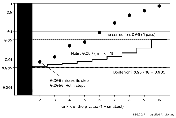
The ten p-values, smallest first, on a log scale. Five pass the uncorrected 0.05. Bonferroni’s flat line at 0.005 and Holm’s rising steps each let only the first through.
On the log scale the two rules look alike at the bottom, where both start at 0.005, and differ at the top, where Holm’s last step reaches the full 0.05. Holm never rejects less.
Build it up
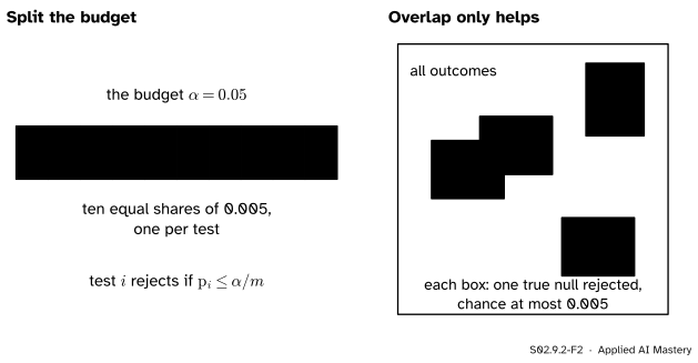
Step 1. Split the budget. Give each of the \(m\) tests the level \(\alpha/m\). With ten tests at 0.05, each p-value must be at most 0.005.
Step 2. Add up the risks. A test of a true null at level \({\alpha/m}\) rejects with chance at most \({\alpha/m}\). The chance that at least one of the true nulls is rejected is the probability of a union, and the union bound of M06.1.4 says it is at most the sum of the chances. Overlap between the events only makes the union smaller than the sum.
S02.9.2-F2
Bonferroni in two pictures. The budget is split equally. The union of the rejection events can cover no more area than the boxes would side by side, and less when they overlap.
Step 3. Spend what is left. Sort the p-values. If the smallest passes \(\alpha/m\), call it a discovery and treat that hypothesis as false. The rest of the family has \({m - 1}\) hypotheses, so the next smallest is held to \({\alpha/(m - 1)}\), the one after to \({\alpha/(m - 2)}\), and so on up to \(\alpha\) itself.
Step 4. Stop at the first failure. The first p-value that misses its step ends the procedure; it and every larger one are kept. This is Holm’s step-down procedure.
The formal statement
Write the p-value of test \(i\) as \(\text{p}_i\), with an upright p to keep it apart from a proportion \(p\), and the sorted values as \({\text{p}_{(1)} \leq \text{p}_{(2)} \leq \dots \leq \text{p}_{(m)}}\), with \(H_{(k)}\) the hypothesis of the \(k\)-th smallest. A valid p-value of a true null satisfies \({\Prob(\text{p}_i \leq u) \leq u}\) for every \(u\) in \([0, 1]\).
NoteBonferroni and Holm
Bonferroni: reject \(H_i\) when \({\text{p}_i \leq \alpha/m}\).
Holm: find the first \(k\) with \({\text{p}_{(k)} > \alpha/(m - k + 1)}\) and reject \({H_{(1)}, \dots, H_{(k-1)}}\); if there is no such \(k\), reject all \(m\).
Both keep \({\text{FWER} \leq \alpha}\), whatever the dependence between the tests.
Bonferroni, proof. Let \(I_0\) be the set of true nulls, with \(m_0\) members. A false positive happens when some \(i\) in \(I_0\) has \({\text{p}_i \leq \alpha/m}\). By the union bound,
No step used independence. The bound is close to tight when the tests are independent and \(\alpha\) is small: for ten independent true nulls the FWER is \({1 - 0.995^{10}} = 0.0489\).
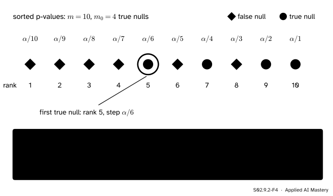
Holm, proof. Look at the true null with the smallest p-value; call its rank \(k^*\). All the hypotheses ranked before it are false nulls, and there are at most \({m - m_0}\) of those, so \({k^* \leq m - m_0 + 1}\). The denominator of its step is therefore
so its step \({\alpha/(m - k^* + 1)}\) is at most \({\alpha/m_0}\).
Holm rejects in order and stops at the first failure, so if it rejects any true null it must reject this first one, which needs \({\text{p}_{(k^*)} \leq \alpha/m_0}\). Hence
The heart of Holm’s proof, for \({m = 10}\) and \({m_0 = 4}\). However the false nulls fall, the first true null meets a step no larger than \({\alpha/m_0}\).
Holm rejects at least as much. Holm’s first step is \({\alpha/m}\) and the later ones are larger. If \({\text{p}_{(k)} \leq \alpha/m}\), then every smaller p-value also passes its own step, so Holm reaches rank \(k\) and rejects it. Every Bonferroni rejection is a Holm rejection.
Šidák’s cut-off. If the tests are independent, a level \(c\) for each gives \({\text{FWER} = 1 - (1 - c)^{m_0}}\) by the previous lesson. Setting \({1 - (1 - c)^m = \alpha}\) and solving gives \({c = 1 - (1 - \alpha)^{1/m}}\): 0.005116 for ten tests, a hair above 0.005. It needs independence; Bonferroni does not.
Adjusted p-values. Rather than move the cut-off, move the p-values: the adjusted p-value of a hypothesis is the smallest family-wise level at which the procedure would reject it. For Bonferroni, \({\text{p}_i \leq \alpha/m}\) exactly when \({m\,\text{p}_i \leq \alpha}\), so the adjusted value is \({\min(1, m\,\text{p}_i)}\). For Holm, \(H_{(k)}\) is rejected exactly when every earlier step passes, that is when \({(m - j + 1)\,\text{p}_{(j)} \leq \alpha}\) for all \({j \leq k}\). Writing \({a_j = (m - j + 1)\,\text{p}_{(j)}}\),
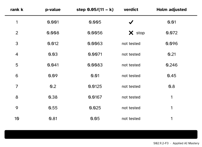
Holm, rank 2: is \({0.008 \leq 0.05/9} = 0.0056\)? No. Stop. One rejection.
Holm adjusted values: \({10 \times 0.001} = 0.01\), then \({9 \times 0.008} = 0.072\), then \({8 \times 0.012} = 0.096\), and so on. At rank 8, \({3 \times 0.38} = 1.14\) is capped at 1, and the running maximum keeps ranks 9 and 10 at 1 although \({1 \times 0.81} = 0.81\).
Šidák’s cut-off 0.005116 also passes only 0.001.
Five p-values were under 0.05, but only one survives the family-wise guarantee. Holm’s extra power shows only when several p-values are small together, as in exercise 1.
Code
The three corrections from scratch, each returning the adjusted p-values in the original order.
Now a check by simulation, 20,000 families of ten one-sided z-tests (seed 4). In the first, every null is true; in the second, the last five hypotheses have a real effect of 3 standard errors.
from scipy import statsdef holm_rows(p, alpha=0.05):"""Holm's rejections for every row of a matrix of p-values at once."""return np.apply_along_axis(holm, 1, p) <= alpharng = np.random.default_rng(4)z = rng.normal(size=(20_000, 10))p_null = stats.norm.sf(z) # all ten nulls truez[:, 5:] +=3# five real effectsp_mix = stats.norm.sf(z)print("all null: FWER none", np.mean((p_null <= alpha).any(1)), " Bonferroni", np.mean((p_null <= alpha / m).any(1)))bon, hol = p_mix <= alpha / m, holm_rows(p_mix)print("five real: FWER Bonferroni", bon[:, :5].any(1).mean(), " Holm", hol[:, :5].any(1).mean())print("real effects found: Bonferroni", bon[:, 5:].sum(1).mean(), " Holm", hol[:, 5:].sum(1).mean())
all null: FWER none 0.40505  Bonferroni 0.04995
five real: FWER Bonferroni 0.0247  Holm 0.0371
real effects found: Bonferroni 3.3198  Holm 3.5321
With every null true, no correction errs in about 40 percent of families and Bonferroni in about 5 percent (0.0489 in theory). With five real effects, both stay under 0.05 (Bonferroni about 0.025, since only five nulls are true, and Holm about 0.037), and Holm finds about 3.5 of the five real effects against Bonferroni’s 3.3. SciPy has no Holm function; the next lesson’s scipy.stats.false_discovery_control covers the false discovery rate instead.
Explore
The many-tests simulator is in lesson S02.9.3. Load the ten p-values there and compare Bonferroni’s flat line with Holm’s steps; then set 50 tests with 40 percent real effects of size 3 and watch Holm’s count pull ahead of Bonferroni’s.
Pitfalls
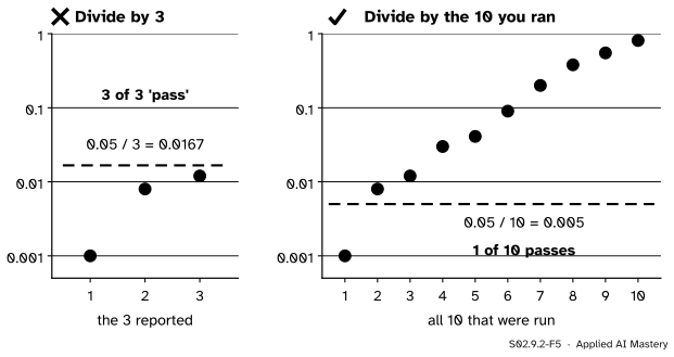
S02.9.2-F5
Wrong beside right. Reporting the three smallest p-values and correcting for three makes all of them “significant”. The family is the ten tests that were run.
“I report three features, so I divide by three.”
The selection already used the other seven p-values: the three were chosen because they were small. The correction must count every test that was run, and with ten that leaves one discovery, not three.
“Bonferroni assumes the tests are independent.”
It assumes nothing about dependence; its proof uses only the union bound. Šidák’s slightly larger cut-off is the one that needs independence. Under strong positive dependence Bonferroni is conservative: its FWER falls well below \(\alpha\).
“Holm’s adjusted p-value is just \({(m - k + 1)\,\text{p}_{(k)}}\).”
Without the running maximum the adjusted values can go down as the raw ones go up: the ten p-values would give 1.14, 1.1 and 0.81 at ranks 8 to 10, so the largest p-value would look the strongest. The maximum over \({j \leq k}\) encodes “stop at the first failure”.
Check yourself
Recall
1. What is Bonferroni’s cut-off for \(m\) tests at family-wise level \(\alpha\), and what is it for the ten p-values?
Show answer
\({\alpha/m}\); \({0.05/10} = 0.005\), which only 0.001 passes.
2. Which inequality proves that Bonferroni controls the FWER, and does the proof need independence?
Show answer
The union bound: the chance of a union is at most the sum of the chances. No independence is needed.
3. In Holm’s procedure, what is the \(k\)-th smallest p-value compared with, and when does the procedure stop?
Show answer
With \({\alpha/(m - k + 1)}\). It stops at the first p-value that is larger than its step.
4. Why does Holm never reject less than Bonferroni?
Show answer
Its steps are all at least \({\alpha/m}\), so any p-value that passes \({\alpha/m}\) is reached and passes its own step, as do all smaller ones.
5. What is the Bonferroni adjusted p-value of 0.008 among ten tests?
Show answer
\({\min(1, 10 \times 0.008)} = 0.08\).
Exercises
1.★ Four tests give p-values 0.004, 0.011, 0.019 and 0.30. At family-wise level 0.05, which hypotheses do Bonferroni and Holm reject?
Show solution
Bonferroni’s cut-off is \({0.05/4} = 0.0125\): it rejects 0.004 and 0.011, two hypotheses.
Holm: \({0.004 \leq 0.05/4} = 0.0125\), reject; \({0.011 \leq 0.05/3} = 0.0167\), reject; \({0.019 \leq 0.05/2} = 0.025\), reject; \({0.30 > 0.05}\), stop. Holm rejects three: the third p-value is too big for Bonferroni but small enough once two hypotheses have been set aside.
2.★★ Compute the Holm adjusted p-values for exercise 1 and check that they give the same decisions.
Show solution
The products \({(m - k + 1)\,\text{p}_{(k)}}\) are \({4 \times 0.004} = 0.016\), \({3 \times 0.011} = 0.033\), \({2 \times 0.019} = 0.038\) and \({1 \times 0.30} = 0.30\). They already increase, so the running maximum leaves them alone: 0.016, 0.033, 0.038 and 0.30. The first three are at most 0.05, the same three rejections.
3.★★★ Show that Šidák’s cut-off is never smaller than Bonferroni’s: \({1 - (1 - \alpha)^{1/m}} \geq {\alpha/m}\) for \(\alpha\) in \([0, 1]\) and \(m \geq 1\).
Show solution
Bernoulli’s inequality (exercise 3 of S02.9.1) with \(\alpha/m\) in place of \(\alpha\) gives
Both sides are at least 0, and taking the \(m\)-th root keeps the order: \({1 - \alpha/m} \geq {(1 - \alpha)^{1/m}}\). Rearranging, \({1 - (1 - \alpha)^{1/m}} \geq {\alpha/m}\). For ten tests at 0.05 the two are 0.005116 and 0.005: the price of making no assumption about dependence is tiny.
Summary card
Share the budget \(\alpha\) among the tests; Holm re-spends what the rejected ones release.
S02.9.2-F1
One rejection each.
Bonferroni. Reject when \({\text{p}_i \leq \alpha/m}\); adjusted \({\min(1, m\,\text{p}_i)}\).
Holm. Compare \({\text{p}_{(k)}}\) with \({\alpha/(m - k + 1)}\), stop at the first failure.
Guarantee.\({\text{FWER} \leq \alpha}\) for both, by the union bound, for any dependence.
Šidák.\({1 - (1 - \alpha)^{1/m}}\), for independent tests only.
Sources and next steps
Sources. Each was opened and checked against this lesson on 15 November 2026.
Siva Balakrishnan, Lecture 23, 36-705 Intermediate Statistics, Carnegie Mellon University, Fall 2019. Section 23.2.2 derives Šidák’s cut-off \({1 - (1 - \alpha)^{1/d}}\) under independence; Section 23.2.3 proves Bonferroni’s control of the FWER from the union bound; Section 23.3 states Holm’s procedure, proves its control by the first-true-null argument used here, and notes that it needs no independence and dominates Bonferroni.
Philip B. Stark, Ninth set of notes: Multiplicity, Statistics 210B, University of California, Berkeley. Section 1 defines the family-wise error rate and strong control; Section 2.1 states Holm’s sequentially rejective method, proves that it controls the FWER (Theorem 1) and describes it as a step-down procedure.