If the labels do not matter, every shuffle of them was equally likely, so rank the observed statistic among the shuffled ones. The two page designs by complete enumeration (38 of 252 splits, p-value 0.151), Monte Carlo shuffles with the (b + 1) / (K + 1) rule derived, and a correlation on the diabetes table.
S02.8.3L2 Intermediate25 minIn review (what this means)
The maths and code on this page are checked by automated tests on every change, but an independent reader has not signed it off yet. Spot a mistake or a confusing step? Tell us.
State the null hypothesis of a permutation test as exchangeability of the labels, and say what it assumes.
Compute an exact permutation p-value by listing every relabelling, and a Monte Carlo one from K random shuffles.
Derive the (b + 1) / (K + 1) rule from treating the observed labelling as one more shuffle.
Run scipy.stats.permutation_test for two groups and for a correlation, choosing the right permutation_type, including for paired data.
The question
Five visitors shown design A spent 4, 5, 7, 8 and 11 minutes on a page; five shown design B spent 6, 9, 10, 12 and 13 (invented, the two designs of S02.7). B is ahead by 3 minutes. The t-test of S02.7.1 assumes the times are roughly normal, and with five per group we cannot check that. Is there a test that assumes nothing about the shape of the data, only that the designs were handed out at random?
From the last lesson
1. The replicates of a statistic \({\hat\theta = 10}\) have \({q^*_{0.025} = 6.22}\) and \({q^*_{0.975} = 15.56}\). What are the percentile and basic 95 percent intervals?
Show answer
Percentile: 6.22 to 15.56. Basic: \({2 \times 10 - 15.56 = 4.44}\) to \({2 \times 10 - 6.22 = 13.78}\).
2. Why can a bootstrap percentile interval for a population maximum almost never cover it?
Show answer
No replicate can exceed the sample’s own maximum, and the sample maximum is below the population maximum unless the sample caught that one value.
Intuition
Suppose the design made no difference at all: each visitor would have spent the same time on whichever page they were shown. Then the labels A and B are just stickers that the randomisation happened to put on the ten times. Any other way of sticking five A’s and five B’s on them was just as likely.
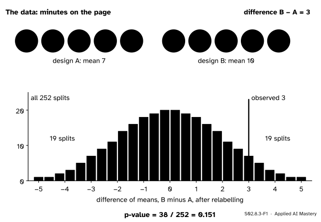
So list every way. There are \({\binom{10}{5} = 252}\) ways to choose which five times get the B sticker. For each, compute B’s mean minus A’s mean. If the real difference, 3, sits far out in that list, the labels probably did matter.
S02.8.3-F1
The permutation distribution of the two designs: the difference of means for all 252 relabellings. Thirty-eight of them, 19 in each tail, are at least as far from 0 as the observed 3.
The p-value is the share of relabellings at least as extreme as the one observed: \({38/252 = 0.151}\). That is not small. A difference of 3 minutes, or more, turns up in 15 percent of random labellings even when the design does nothing.
Build it up
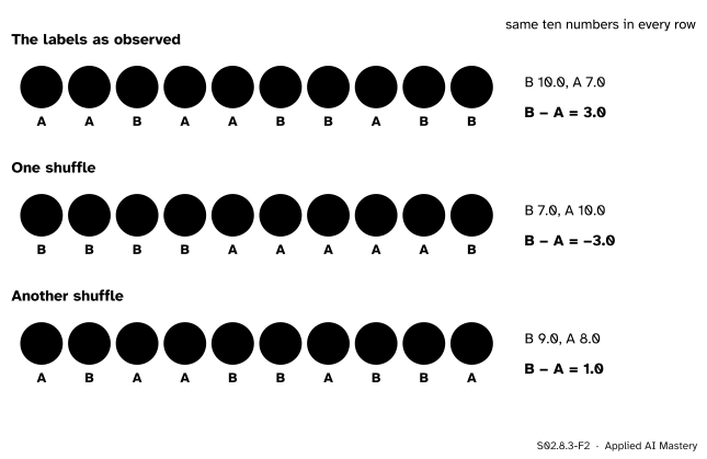
Step 1. Keep the data, move the labels. The ten times never change. A permutation, or shuffle, deals the ten labels out again at random, five of each.
S02.8.3-F2
Two shuffles of the labels. The ten numbers stay put; only which five count as B changes, and with it the difference of means.
Step 2. Recompute the statistic. For each shuffle compute the same test statistic\(T\) as for the real data, here B’s mean minus A’s. The first shuffle in the figure gives \({-3}\), as far from 0 as the observed 3 but on the other side.
Step 3. Rank the observed value. Collect \(T\) over all shuffles: this is the permutation distribution, the null distribution of S02.5 built by relabelling. Count the shuffles with \({\abs{T} \ge 3}\) for a two-sided test.
Step 4. When there are too many shuffles to list, sample them. Ten values split five and five give 252 shuffles; 442 patients give more than \({10^{900}}\) orderings. Then draw \(K\) random shuffles and count among them, with one correction derived below.
The formal statement
NoteDefinition: a permutation test
Random variables are exchangeable if their joint distribution does not change when they are reordered. A permutation test of two groups takes as its null hypothesis that all the observations are exchangeable: the group labels carry no information. Given the pooled values, every one of the \({\binom{n_1 + n_2}{n_1}}\) ways to assign the labels is then equally likely, so the exact p-value is
where \(N_{\text{extreme}}\) is the number of labellings with \({\abs{T} \ge \abs{T_{\text{obs}}}}\).
Random assignment is what makes the null distribution right: the experimenter really did choose one labelling of 252 at random, so under \({H_0}\) the observed one is a uniform draw from the list. No normality, no large-sample approximation.
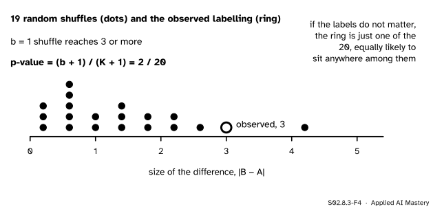
Monte Carlo shuffles. Draw \(K\) labellings at random and let \(b\) be the number with \({\abs{T} \ge \abs{T_{\text{obs}}}}\). Call the observed statistic \(T_0\) and the shuffled ones \({T_1, \dots, T_K}\). Under \({H_0}\) all \({K + 1}\) labellings are independent uniform draws from the same list, so the \({K + 1}\) values are exchangeable, and (if there are no ties) the observed one is equally likely to hold any of the \({K + 1}\) ranks. Its rank from the top is \({1 + b}\), so
A small \(b\) is the evidence against \({H_0}\), so this probability is the p-value:
\[
\text{p-value} = \frac{b + 1}{K + 1}.
\]
The test that rejects when this is at most \(\alpha\) rejects a true \({H_0}\) with probability \({\lfloor \alpha(K+1) \rfloor/(K+1) \le \alpha}\), so it keeps its promise for every \(K\). With ties the p-value is a little larger than it needs to be, which errs on the safe side. The tempting \({b/K}\) can be exactly 0, a claim that the data are impossible under \({H_0}\), which a random sample of shuffles can never show.
S02.8.3-F4
Nineteen random shuffles and the observed labelling. Under the null hypothesis the ring is one of 20 exchangeable values, so its rank among them is uniform: hence \({(b + 1)/(K + 1)}\).
Go deeper: what exchangeability does and does not cover
A permutation test is exact for the hypothesis that the labels do not matter at all: the two groups have the same distribution. It is not a test that the means are equal while the spreads differ. If design B made times more variable without changing their mean, shuffling would still see a difference in the data, because pooling the two groups is only fair when their distributions agree. Hesterberg lists this among the limits of permutation tests: equality of means when the variances may differ, and a single-sample mean, which has no labels to shuffle.
Worked example
Counting the 38 by hand. The ten times add to 85. If the five B times add to \(S\), then the five A times add to \({85 - S}\), and
So \({T \ge 3}\) exactly when \({2S - 85 \ge 15}\), that is \({S \ge 50}\): we need the ways to choose five of the ten times adding to at least 50. The largest is \({9 + 10 + 11 + 12 + 13 = 55}\). Work down from there.
S02.8.3-F3
The upper tail counted by B’s total: \({1 + 1 + 2 + 3 + 5 + 7 = 19}\) splits. The observed split is one of the seven with total 50.
Totals 55 and 54 can each be made one way; 53 two ways; 52 three; 51 five; 50 seven, one of them the observed split. That is 19 splits with \({T \ge 3}\). Swapping every A for a B turns \(T\) into \({-T}\), so 19 more have \({T \le -3}\). The two-sided p-value is \({38/252 = 0.151}\) and the one-sided one \({19/252 = 0.075}\).
Compare the t-test of S02.7.1 on the same data: p-value 0.122. The two need not agree, because the t-test leans on a normal model and the permutation test only on the random assignment. Neither gives strong evidence that design B holds visitors longer.
Code
Complete enumeration with itertools, then random shuffles with rng.permuted:
import itertoolsimport numpy as npfrom scipy import statsa = np.array([4, 5, 7, 8, 11], dtype=float) # design A, minutes (invented)b = np.array([6, 9, 10, 12, 13], dtype=float) # design Btimes = np.concatenate([a, b])observed = b.mean() - a.mean()diffs = []for chosen in itertools.combinations(range(10), 5): # which five get the B label is_b = np.zeros(10, dtype=bool) is_b[list(chosen)] =True diffs.append(times[is_b].mean() - times[~is_b].mean())diffs = np.array(diffs)extreme =int(np.sum(np.abs(diffs) >=abs(observed) -1e-9))print(len(diffs), "splits;", extreme, "at least as extreme; p-value", round(extreme /len(diffs), 3))K =999rng = np.random.default_rng(0)shuffled = rng.permuted(np.tile(times, (K, 1)), axis=1) # each row: the ten times in a random ordert_star = shuffled[:, 5:].mean(axis=1) - shuffled[:, :5].mean(axis=1)b_count =int(np.sum(np.abs(t_star) >=abs(observed) -1e-9))print(f"{b_count} of {K} shuffles; p-value (b + 1)/(K + 1) = {(b_count +1) / (K +1):.3f}")
252 splits; 38 at least as extreme; p-value 0.151
143 of 999 shuffles; p-value (b + 1)/(K + 1) = 0.144
The Monte Carlo answer, 0.144, is close to the exact 0.151; its own noise is about \({\sqrt{0.15 \times 0.85 / 1000} = 0.011}\). SciPy computes the exact test by itself when the number of distinct shuffles is at most n_resamples:
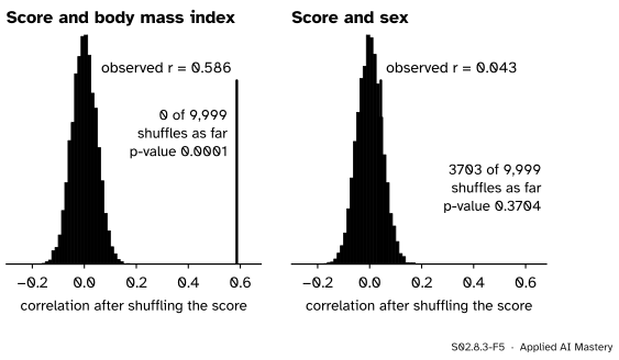
A correlation. To test whether body mass index and the progression score of the diabetes table are related, shuffle one column against the other: under \({H_0}\) of no relation, any pairing was as likely as the observed one. In scipy this is permutation_type="pairings".
from sklearn.datasets import load_diabetestable = load_diabetes(as_frame=True, scaled=False).framescore = table["target"].to_numpy(float)def corr(x, y, axis=-1): dx = x - x.mean(axis=axis, keepdims=True) dy = y - y.mean(axis=axis, keepdims=True)return (dx * dy).sum(axis=axis) / np.sqrt((dx **2).sum(axis=axis) * (dy **2).sum(axis=axis))K =9999shuffled = np.random.default_rng(0).permuted(np.tile(score, (K, 1)), axis=1)found = {}for column in ("bmi", "sex"): x = table[column].to_numpy(float) r = corr(x, score) count =int(np.sum(np.abs(corr(x[None, :], shuffled, axis=1)) >=abs(r) -1e-12)) # ties count lib = stats.permutation_test((x, score), corr, permutation_type="pairings", vectorized=True, rng=np.random.default_rng(0)) found[column] = (r, count, (count +1) / (K +1), lib.pvalue)print(f"{column}: r = {r:.3f}, {count} of {K} shuffles as far, p-value {(count +1) / (K +1):.4f}, "f"scipy {lib.pvalue:.4f}")
bmi: r = 0.586, 0 of 9999 shuffles as far, p-value 0.0001, scipy 0.0002
sex: r = 0.043, 3703 of 9999 shuffles as far, p-value 0.3704, scipy 0.3770
S02.8.3-F5
Body mass index: no shuffle comes anywhere near the observed correlation, so the p-value is the smallest that 9,999 shuffles can give, 1/10,000. Sex: a correlation of 0.043 is ordinary among shuffles.
No shuffle comes within 0.39 of the body-mass-index correlation, so \({b = 0}\) and the p-value is \({1/10{,}000}\), not 0. SciPy reports 0.0002 because its two-sided p-value is twice the smaller one-sided one, a convention its documentation notes is not universal. Sex takes only two values, so a few shuffles tie the observed correlation exactly; the code compares with a tiny tolerance so that rounding in the last digit cannot drop a tie from the count.
Explore
Open the resampling machine in lesson S02.8.1 and switch to Shuffle the designs. Each step deals the A and B labels out again and drops the new difference onto the null distribution; watch the share beyond 3 settle towards 38/252.
Pitfalls
“None of my 9,999 shuffles beat the data, so the p-value is 0.”
Zero would mean the observed labelling is impossible under \({H_0}\), and the observed labelling is always one of the possible ones. Report \({(b + 1)/(K + 1)}\), here \({1/10{,}000}\), and say that it is the smallest value the run could give. Phipson and Smyth show that reporting \({b/K}\) inflates false positives, badly so when thousands of tests are run (S02.9).
S02.8.3-F6
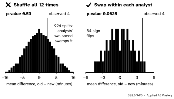
Wrong beside right, on the new tool of S02.7 (six analysts timed with both tools). Shuffling all twelve times mixes fast and slow analysts; swapping only within each analyst keeps the pairs.
“Shuffle all the values, whatever the design.”
The shuffle must copy how the data were made. The six analysts each used both tools, so under \({H_0}\) the only thing chance decided is which of each analyst’s two times carries which label. Swapping within pairs flips the sign of each difference (\({2^6 = 64}\) ways): 4 of the 64 give a mean difference as large as 4, p-value 0.0625. Shuffling all twelve times freely ignores the pairing and gives 0.53, the same mistake as the unpaired t-test of S02.7.1. In scipy, paired data take permutation_type="samples".
“A permutation test needs no assumptions at all.”
It needs exchangeability under \({H_0}\): random assignment, or rows that are independent and identically distributed. Rows that come in clusters (several visits by one user) or in time order are not exchangeable, and shuffling them one at a time understates the noise, exactly as for the bootstrap of S02.8.2.
Check yourself
Recall
1. What is the null hypothesis of a two-group permutation test?
Show answer
That the observations are exchangeable: the labels carry no information, so every assignment of labels to the pooled values was equally likely.
2. How many ways are there to split ten values five and five, and how many of them are at least as extreme as the two designs’ difference of 3?
Show answer
\({\binom{10}{5} = 252}\), of which 38 (19 in each tail), so the p-value is 0.151.
3. With \(K\) random shuffles of which \(b\) are at least as extreme, what p-value is reported, and why?
Show answer
\({(b + 1)/(K + 1)}\): under \({H_0}\) the observed statistic is one of \({K + 1}\) exchangeable values, so its rank is uniform, and \({\Prob(B \le b) = (b + 1)/(K + 1)}\).
4. What do you shuffle to test a correlation, and which permutation_type does that?
Show answer
One column against the other, breaking the pairing of rows: permutation_type="pairings".
5. How are paired data shuffled?
Show answer
Within each pair only, which flips the sign of each difference: permutation_type="samples".
Exercises
1.★ A permutation test with \({K = 4{,}999}\) shuffles finds \({b = 12}\) at least as extreme. Give the p-value, and the smallest p-value this run could have produced.
The smallest possible, with \({b = 0}\), is \({1/5{,}000} = 0.0002\).
2.★★ Groups A = {1, 2} and B = {3, 5}. List every split of the four values into two pairs, compute B’s mean minus A’s for each, and find the two-sided permutation p-value.
Show solution
There are \({\binom{4}{2} = 6}\) choices for B. The values add to 11, so with B’s total \(S\) the difference is \({S/2 - (11 - S)/2 = S - 5.5}\). B = {1, 2}: \({-2.5}\). {1, 3}: \({-1.5}\). {1, 5}: 0.5. {2, 3}: \({-0.5}\). {2, 5}: 1.5. {3, 5}: 2.5, the observed. Two of the six have \({\abs{T} \ge 2.5}\), so the p-value is \({2/6 = 0.333}\). With two per group, no result could give a p-value below 1/3.
3.★★★ With \({K = 20}\) shuffles and level \({\alpha = 0.05}\), compute the chance, under \({H_0}\) and with no ties, that a test rejects when it uses \({b/K}\), and when it uses \({(b + 1)/(K + 1)}\).
Show solution
Under \({H_0}\), \(B\) is uniform on \({0, 1, \dots, 20}\), each value with probability 1/21. Using \({b/K \le 0.05}\) means \({b \le 1}\), which has probability \({2/21 = 0.095}\): almost twice the promised 5 percent. Using \({(b + 1)/21 \le 0.05}\) means \({b + 1 \le 1.05}\), so \({b = 0}\), with probability \({1/21 = 0.048}\), within the promise.
Summary card
If the labels do not matter, shuffle them, and see where the real labelling ranks.
S02.8.3-F1
38 of 252 splits: p-value 0.151.
Exact. The share of all relabellings with \({\abs{T} \ge \abs{T_{\text{obs}}}}\).
Monte Carlo.\({(b + 1)/(K + 1)}\) from \(K\) random shuffles; never 0.
Shuffle as the data were made: groups, pairs or pairings.
Sources. Each was opened and checked against this lesson on 15 November 2026.
SciPy, scipy.stats.permutation_test: the permutation types 'independent', 'samples' and 'pairings', the exact test when n_resamples is at least the number of distinct permutations, the randomised p-value with one added to numerator and denominator (citing Phipson and Smyth), and the two-sided p-value as twice the smaller one-sided one, a convention it notes is not universal.
Belinda Phipson and Gordon K. Smyth, Permutation p-values should never be zero, Statistical Applications in Genetics and Molecular Biology 9, article 39 (2010). Sections 2 and 3 show that \({b/m}\) raises the type I error rate, seriously so when many tests are run; section 4 derives the exact Monte Carlo p-value \({(b + 1)/(m + 1)}\) from the uniform distribution of the count; section 6 shows that when shuffles are drawn with replacement the exact p-value is slightly smaller than \({(b + 1)/(m + 1)}\); and the abstract warns that \({b/m}\) understates p-values by about \({1/m}\).
Tim Hesterberg, What Teachers Should Know about the Bootstrap, arXiv:1411.5279 (2014). Section 7.3 lists the limits of permutation tests, among them that they cannot test equal means when the variances may differ.