Turn the power formula round to find the sample size before collecting any data: one mean, two means and two proportions, with the exact t-test check by the noncentral t, and why detecting a one-point accuracy gain needs about 13,500 test examples per model.
S02.6.3L2 Intermediate25 minIn review (what this means)
The maths and code on this page are checked by automated tests on every change, but an independent reader has not signed it off yet. Spot a mistake or a confusing step? Tell us.
Derive the sample size for a z-test from the power formula, for one mean and for two means.
Derive and use the sample size per group for comparing two proportions.
Check a normal-formula sample size with the exact power of the t-test from the noncentral t distribution.
Explain why the sample size grows like one over the effect squared, and what that means for comparing models on test sets.
The question
The two page designs were each shown to five visitors. If design B really keeps people 1.095 standard deviations longer, as the sample suggested, that study had only a one-in-three chance of reaching significance. How many visitors per design should the next study plan for, to have an 80 percent chance? And how many test examples does it take to show that a new model’s accuracy of 0.91 beats an old model’s 0.90?
From the last lesson
1. For two groups of \(n\), how is the t statistic built from Cohen’s d?
Show answer
\(t = \hat{\delta}\sqrt{n/2}\), the effect times the square root of half the group size.
2. An error rate falls from 0.10 to 0.09. Give the difference and the relative risk.
Show answer
The difference is one percentage point, \(-0.01\); the relative risk is 0.9.
Intuition
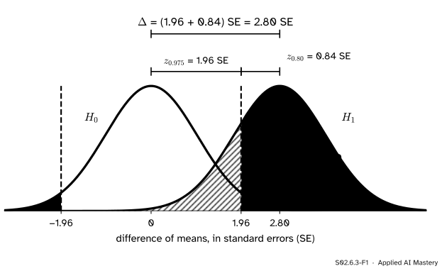
Lesson S02.6.1 started from \(n\) and found the power. Planning runs the other way: fix the power you want and find the \(n\) that delivers it. One picture holds the whole argument.
S02.6.3-F1
The cut-off must sit 1.96 standard errors above the null centre (for a two-sided test at level 0.05) and 0.84 standard errors below the alternative’s centre (so that 80 percent of it lies beyond). The effect must therefore span 2.80 standard errors.
The cut-off is pinned from two sides. The level fixes its distance from the null’s centre. The power fixes its distance from the alternative’s centre. Both distances are counted in standard errors, so the true effect must be \({1.96 + 0.84} = 2.80\) standard errors long. The effect is what it is; the only thing we control is the standard error, and \(n\) shrinks it.
Build it up
Step 1. The level fixes one gap. A two-sided test at level 0.05 puts its cut-off at \(z_{0.975} = 1.96\) standard errors from the null’s centre.
Step 2. The power fixes the other. For the alternative’s bell to have 80 percent of its area beyond the cut-off, the cut-off must sit \(z_{0.80} = 0.84\) standard errors below its centre, because a standard normal is above \(-0.84\) with probability 0.80.
Step 3. Add. The effect must equal \({(1.96 + 0.84)} = 2.80\) standard errors.
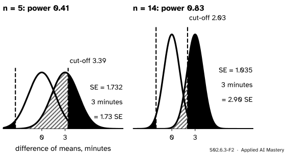
Step 4. Make the standard error fit. For the two designs the standard error of the difference is \({\sigma\sqrt{2/n}}\). With five per group it is 1.732 minutes, and a 3-minute effect is only 1.73 standard errors. With 14 per group it is 1.035, and 3 minutes is 2.90 standard errors: enough.
S02.6.3-F2
The same 3-minute effect with 5 and with 14 visitors per design (normal approximation). The effect does not move; the bells narrow until it spans more than 2.80 standard errors.
The formal statement
One mean. Start from the two-sided power, dropping the far tail, which is tiny once the power is useful (it was 0.0001 in S02.6.1):
Round \(n\) up: rounding down gives less than the power asked for. A one-sided test uses \(z_{1-\alpha}\) in place of \(z_{1-\alpha/2}\).
Two means. With \(n\) per group the standard error is \({\sigma\sqrt{2/n}}\). The same steps give twice as many per group, and only \(\delta = \Delta/\sigma\) matters:
\[
n \text{ per group} = 2\Big(\frac{z_{1-\alpha/2} + z_{1-\beta}}{\delta}\Big)^2 .
\]
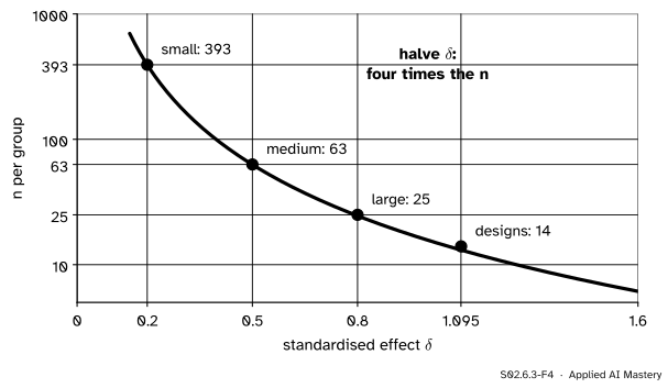
The effect sits in the denominator, squared: halve \(\delta\) and \(n\) quadruples.
S02.6.3-F4
Sample size per group for 80 percent power at level 0.05, two-sided. A small effect needs 393 per group; a large one, 25.
Two proportions. For proportions \(p_1\) and \(p_2\) in two groups of \(n\), the variance of \({\hat{p}_2 - \hat{p}_1}\) is \({(p_1(1-p_1) + p_2(1-p_2))/n}\), so the standard error takes the place of \({\sigma\sqrt{2/n}}\) and
Some books use the pooled proportion under \(H_0\) for the first \(z\). The answer barely moves: for the accuracy example below it goes from 13,493 to 13,495.
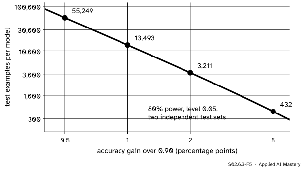
S02.6.3-F5
How many test examples each of two models needs to show an accuracy gain over 0.90. Each halving of the gain multiplies the test set by about four.
The exact t-test. The formulas treat \(\sigma\) as known. When the test estimates it, the t statistic under the alternative follows the noncentral t distribution: if \(Z\) is standard normal and \(V\) an independent \(\chi^2_\nu\), then \({T = (Z + \lambda)/\sqrt{V/\nu}}\) has the noncentral t distribution with \(\nu\) degrees of freedom and noncentrality \(\lambda\). For the pooled two-sample test, \(\nu = 2n - 2\) and \(\lambda = \delta\sqrt{n/2}\) (stated here, not derived). The exact power is \({\Prob(T \ge t_c)} + {\Prob(T \le -t_c)}\), with \(t_c = t_{\nu, 0.975}\). SciPy calls this distribution scipy.stats.nct.
Worked example
The two designs.\(\delta = 1.095\), level 0.05 two-sided, power 0.80.
S02.6.3-F3
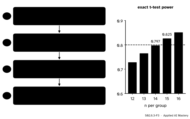
The normal formula in four steps, then the exact check. Fourteen per group falls just short of 0.80 with the t-test; fifteen clears it.
Square and double: \({2 \times 2.557^2} = 13.08\).
Round up: 14 per group by the normal formula.
Now the exact check. At \(n = 14\) the t-test has \(\nu = 26\), \(\lambda = {1.095 \times \sqrt{7}} = 2.898\), and the noncentral t gives power 0.797, a hair short. At \(n = 15\), \(\nu = 28\) and \(\lambda = 3.000\), and the power is 0.825. So 15 per group, against the 5 the study had: at \(n = 5\) the same calculation gives 0.33. The t-test needs a little more than the normal formula because estimating \(\sigma\) costs some precision.
Accuracy on test sets. Two models are scored on separate test sets, and the gain to detect is 0.90 to 0.91. With \({p_1(1-p_1) + p_2(1-p_2)} = {0.09 + 0.0819} = 0.1719\),
so 13,493 test examples per model, about 13,500. A one-point gain is a small effect on a proportion near 0.9, and small effects need big samples. This is why online A/B tests of a change that moves a rate by a fraction of a point run for weeks (S05.3). Scoring both models on the same test examples is a paired design and usually needs far fewer (S02.7).
Code
From scratch, with quantiles from the standard library:
two designs: 13.08 -> 14 per group
accuracy 0.90 -> 0.905: 55,249 per model
accuracy 0.90 -> 0.910: 13,493 per model
accuracy 0.90 -> 0.920: 3,211 per model
accuracy 0.90 -> 0.950: 432 per model
The exact power of the t-test, from the noncentral t:
from scipy import statsdef t_power(n, delta, alpha=0.05): df, nc =2* n -2, delta * math.sqrt(n /2) tc = stats.t.ppf(1- alpha /2, df)return stats.nct.sf(tc, df, nc) + stats.nct.cdf(-tc, df, nc)for n in (5, 13, 14, 15, 16):print(n, round(t_power(n, delta), 3))exact_n =next(n for n inrange(2, 100) if t_power(n, delta) >=0.80)print("smallest n with power 0.80:", exact_n)
5 0.333
13 0.764
14 0.797
15 0.825
16 0.85
smallest n with power 0.80: 15
And a check by simulation: 20,000 pairs of normal samples of 15 with the designs’ effect, each tested with scipy.stats.ttest_ind.
import numpy as nprng = np.random.default_rng(3)a = rng.normal(0, 1, size=(20_000, 15))b = rng.normal(delta, 1, size=(20_000, 15))rejected = np.mean(stats.ttest_ind(b, a, axis=1).pvalue <0.05)print("simulated power with 15 per group:", rejected)
simulated power with 15 per group: 0.82455
Explore
The module’s interactive, the power explorer, is in lesson S02.6.1. Its Go to 80% power button jumps to the \(n\) of this lesson’s formula, rounded up. Try \(\delta = 1.095\) (14), then halve it to 0.55 and watch the number roughly quadruple.
Pitfalls
S02.6.3-F6
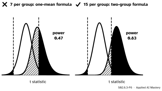
Wrong beside right, by the exact t-test. The one-mean formula gives 6.54, so 7 per group, and only 0.47 power. The two-group formula, checked with the t-test, gives 15 per group and 0.83.
“The formula gave 6.54, so 7 visitors per design.”
That is the one-mean formula, \({((z_{0.975} + z_{0.80})/\delta)^2}\). Comparing two groups doubles the variance of the difference, and so doubles \(n\) per group.
“The formula said 13.08, so 13 will do.”
Always round up, and check small samples with the exact t-test: here 13 gives 0.76 and even 14 gives only 0.797.
“Plan for the effect the pilot study found.”
A small pilot’s effect is a noisy estimate, and a pilot that looked promising enough to follow up probably overestimated it (lesson S02.6.4). Plan for the smallest effect worth acting on.
“Plan n, then stop early if it is significant.”
The power and the level were computed for the planned \(n\). Peeking and stopping early inflates the false-positive rate; S05.5 treats it.
Check yourself
Recall
1. How many standard errors must the effect span for 80 percent power at level 0.05 two-sided?
3. If the effect to detect halves, what happens to \(n\)?
Show answer
It is multiplied by four, because \(n\) grows like \({1/\delta^2}\).
4. Which distribution gives the exact power of the t-test?
Show answer
The noncentral t, with \(2n - 2\) degrees of freedom and noncentrality \(\delta\sqrt{n/2}\).
5. About how many test examples per model detect an accuracy gain from 0.90 to 0.91 with independent test sets?
Show answer
About 13,500 (13,493 by the formula).
Exercises
1.★ The rent test of S02.6.1 is one-sided at level 0.05, with \(\sigma = 5.41\) and a rise of 2 to detect. How many flats give 80 percent power?
Show solution
One mean, one-sided: \({n = ((1.645 + 0.842) \times 5.41/2)^2} = (6.726)^2 = 45.24\), so 46 flats. (Two-sided, with 1.96, it would be 57.43, so 58.)
2.★★ Plan the designs study for 90 percent power at level 0.05 two-sided, first by the normal formula and then by the exact t-test, given that the t-test’s power is 0.891 at 18 per group and 0.907 at 19.
Show solution
\(z_{0.90} = 1.282\), so \({n = 2((1.960 + 1.282)/1.095)^2} = 17.51\), and the normal formula says 18. The exact t-test has 0.891 at 18, short of 0.90, and 0.907 at 19, so 19 per group.
3.★★★ Derive the sample size per group for two proportions from the power formula, and use it to plan a test of a conversion rate rising from 0.80 to 0.85.
Show solution
Write \(q = 1 - p\). \(\hat{p}_1\) and \(\hat{p}_2\) are independent with variances \({p_1 q_1/n}\) and \({p_2 q_2/n}\), so the variances add and \({\hat{p}_2 - \hat{p}_1}\) has standard error
Here \({p_1 q_1 + p_2 q_2} = {0.16 + 0.1275} = 0.2875\), so \({n = 7.849 \times 0.2875/0.0025} = 902.6\): 903 per group.
Summary card
Choose n so the effect spans 2.80 standard errors.
S02.6.3-F1
1.96 plus 0.84 equals 2.80.
One mean.\(n = {((z_{1-\alpha/2} + z_{1-\beta})\sigma/\Delta)^2}\), rounded up.
Two means.\(n\) per group \(= {2((z_{1-\alpha/2} + z_{1-\beta})/\delta)^2}\).
Two proportions. Replace \({2\sigma^2}\) by \({p_1 q_1 + p_2 q_2}\) and \(\Delta\) by \({p_2 - p_1}\).
Small n. Check with the noncentral t: the designs need 15, not 14.
Sources and next steps
Sources. Each was opened and checked against this lesson on 15 November 2026.
David Diez, Mine Çetinkaya-Rundel and Christopher Barr, OpenIntro Statistics, 4th edition (free PDF). Section 7.4.3, “Determining a proper sample size”, draws the null and alternative distributions, notes that the rejection region sits 1.96 standard errors from the null and that 80 percent power puts the alternative’s centre 0.84 standard errors beyond it, and solves \({0.84\,\mathrm{SE} + 1.96\,\mathrm{SE} = 2.8\,\mathrm{SE}}\) for the size per group.
SciPy, scipy.stats.nct. Defines the noncentral t as \({(Y + c)/\sqrt{V/k}}\) with \(Y\) standard normal and \(V\) an independent chi-square on \(k\) degrees of freedom, with shape parameters df and nc.