Fix a level alpha before the data arrive and a p-value becomes a yes-or-no decision. Draw the overlap diagram of the null and alternative distributions, read off the Type I and Type II error rates, and see the same trade in a classifier’s threshold.
S02.5.3L2 Intermediate25 minIn review (what this means)
The maths and code on this page are checked by automated tests on every change, but an independent reader has not signed it off yet. Spot a mistake or a confusing step? Tell us.
Turn a p-value into a decision with a level alpha fixed in advance, and write the rejection region of a one- or two-sided z-test.
Define Type I and Type II errors, and show that a level-alpha test makes a Type I error with probability alpha.
Derive the Type II error rate of the one-sided z-test for a given alternative (0.20 for the listing site against a true mean of 11).
Explain how moving the critical value trades one error for the other, and relate it to a classifier’s threshold.
The question
A spam filter must decide, an alarm must ring or stay quiet, a new model must ship or not. A p-value is a number between 0 and 1, not a decision. How do you turn it into a yes or a no, and how often will that yes or no be wrong?
From the last lesson
1. Define the p-value in one sentence.
Show answer
The probability, computed as if \(H_0\) were true, of a test statistic at least as extreme as the one observed.
2. What is the distribution of a continuous test’s p-value when \(H_0\) is true?
Show answer
Uniform on \({[0, 1]}\), so \({\Prob(P \le u) = u}\) for every \(u\).
Intuition
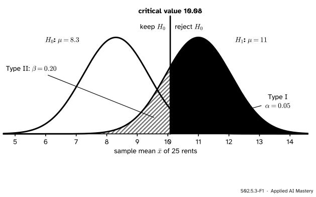
Go back to the listing site of the last lesson, whose 25 flats have a mean rent of 10.5 against the city’s 8.3. This time the question is one-sided: is the site dearer? Before looking, we promise to reject \({H_0 : \mu = 8.3}\) only if \(\bar{x}\) lands so high that a typical site would get there just 5 percent of the time. That fixes a line, and the picture shows what the line costs.
S02.5.3-F1
The overlap diagram. If \(H_0\) is true, \(\bar{x}\) follows the black curve; if the site’s mean is really 11, it follows the blue one. The orange line splits the axis into “keep” and “reject”. The solid area is the chance of rejecting a true \(H_0\); the hatched area is the chance of keeping a false one.
Two curves, one line, two kinds of mistake. Slide the line right and the solid area shrinks while the hatched area grows. Slide it left and the reverse happens. No position removes both, because the curves overlap.
Build it up
Step 1. Choose a level in advance. The significance level\(\alpha\) is the largest chance of a false alarm you will accept, chosen before the data are seen. The usual choice is 0.05; a costly false alarm calls for 0.01. The decision rule is: reject \(H_0\) when the p-value is at most \(\alpha\), otherwise keep it.
Step 2. The rule as a region. For the one-sided z-test the p-value is \({1 - \Phi(z)}\), and
The last step holds because \(\Phi\) is increasing, and \({z_{1-\alpha}}\) is the quantile with \({\Phi(z_{1-\alpha}) = 1 - \alpha}\); for \({\alpha = 0.05}\) it is \({z_{0.95} = 1.645}\). The set of values that lead to rejection is the rejection region. On the scale of \(\bar{x}\) it starts at the critical value\({c = \mu_0 + z_{0.95}\,\sigma/\sqrt{n}}\), which is \({8.3 + 1.645 \times 1.082 = 10.08}\).
Step 3. Two-sided. The two-sided p-value is at most \(\alpha\) exactly when \({\abs{z} \ge z_{1-\alpha/2}}\), which is 1.96 for \({\alpha = 0.05}\). On the scale of \(\bar{x}\) we keep \(H_0\) between \({8.3 - 2.12 = 6.18}\) and \({8.3 + 2.12 = 10.42}\) and reject outside.
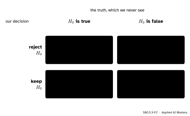
Step 4. Four outcomes. The truth is \(H_0\) or not; our decision is reject or keep. Two of the four combinations are mistakes.
S02.5.3-F2
The four outcomes of a test. A Type I error rejects a true \(H_0\); a Type II error keeps a false one. We choose \(\alpha\); \(\beta\) follows from the design and the truth.
The court analogy helps. \(H_0\) is “innocent”. Convicting an innocent person is a Type I error; acquitting a guilty one is a Type II error. A court that demands proof beyond reasonable doubt chooses a small \(\alpha\), and pays for it with more guilty people walking free.
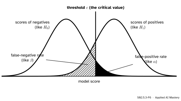
Step 5. The same picture in machine learning. A classifier scores each email and flags it as spam when the score passes a threshold \(c\) (ML01.6.4). The scores of genuine emails and of spam are two overlapping distributions, exactly like the two curves above.
S02.5.3-F6
A classifier’s threshold is a critical value. Negatives scored above it are false positives (the Type I area); positives scored below it are false negatives (the Type II area).
The false-positive rate is \(\alpha\) and the false-negative rate is \(\beta\). Raising the threshold cuts false alarms and misses more spam. The ROC curve of ML01.7.3 draws every such trade at once.
The formal statement
NoteDefinitions
A test at level \(\alpha\) rejects \(H_0\) when the p-value is at most \(\alpha\).
Type I error: rejecting \(H_0\) when it is true. \({\Prob(\text{reject} \mid H_0) = \alpha}\).
Type II error: keeping \(H_0\) when it is false. Its rate is \(\beta\), which depends on which alternative is true.
Power:\({1 - \beta}\), the chance of rejecting a false \(H_0\) (the subject of S02.6).
Why the Type I rate is exactly \(\alpha\). Under \(H_0\) the statistic \({Z}\) follows \({N(0, 1)}\), so for the one-sided test
The same follows from the last lesson: a p-value that is uniform under \(H_0\) is at most \(\alpha\) with chance \(\alpha\). For a count the p-value is only “at most uniform”, so the Type I rate is at most \(\alpha\).
The Type II rate for one alternative. Suppose the truth is \({\mu = \mu_1}\) with \({\mu_1 > \mu_0}\). Then \({\bar{x} \sim N(\mu_1, \mathrm{SE}^2)}\), where \({\mathrm{SE} = \sigma/\sqrt{n}}\). We keep \(H_0\) when \({\bar{x} < c}\), so
The second line standardises \(\bar{x}\) with the alternative’s mean. The third substitutes \({c = \mu_0 + z_{1-\alpha}\,\mathrm{SE}}\) and splits the fraction. The formula shows every lever at once: a farther alternative, a smaller \(\mathrm{SE}\) (more data) or a larger \(\alpha\) each make \(\beta\) smaller. S02.6 builds on it.
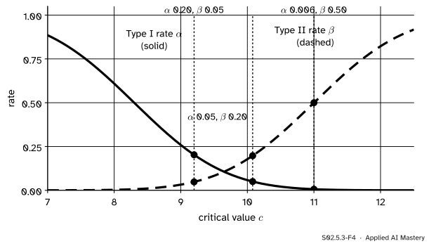
The trade. Fix the data and move \(c\). The Type I rate \({1 - \Phi((c - \mu_0)/\mathrm{SE})}\) falls as \(c\) rises; the Type II rate \({\Phi((c - \mu_1)/\mathrm{SE})}\) rises. One can be bought only with the other.
S02.5.3-F4
Moving the critical value for the listing site, with the alternative \({\mu_1 = 11}\). At \({c = 9.2}\), \({\alpha = 0.20}\) and \({\beta = 0.05}\); at 10.08, 0.05 and 0.20; at 11, 0.006 and 0.50.
Go deeper: why fix alpha and not beta
The two hypotheses are not treated alike. \(H_0\) is a single precise value, so the Type I rate is a single number we can set. The alternative is usually a range (\({\mu > 8.3}\)), and \(\beta\) is a different number for each value in it: 0.84 if the truth is 9, 0.20 if it is 11, almost 0 if it is 14. So the convention is to cap the error we can compute exactly, the false alarm, and to study \(\beta\) as a curve over the alternatives. That curve, read as power, is the subject of S02.6.
Worked example
At level 0.05, is the listing site dearer than the city? And how often would this test miss a site whose true mean is 11?
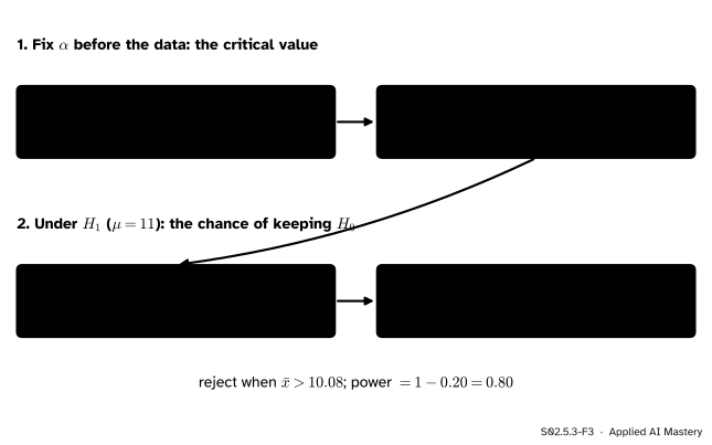
S02.5.3-F3
The critical value comes from \(\alpha\) and \(H_0\) alone; \(\beta\) needs a specific alternative.
Level and region.\({\alpha = 0.05}\), one-sided, so \({z_{0.95} = 1.645}\) and \({c}\)\({= 8.3 + 1.645 \times 1.082}\)\({= 8.3 + 1.780}\)\({= 10.08}\). Reject when \({\bar{x} > 10.08}\).
Decision. The site’s \({\bar{x} = 10.5}\) is above 10.08, so we reject \(H_0\). The p-value route agrees: \({0.021 \le 0.05}\). Had we chosen \({\alpha = 0.01}\) the critical value would be 10.82 and we would keep \(H_0\) (exercise 1). The data are the same; the decision depends on a level fixed in advance, which is why it must be fixed in advance.
Type II rate at \({\mu_1 = 11}\). Standardise the critical value with the alternative’s mean: \({(10.08 - 11)/1.082 = -0.85}\), so \({\beta = \Phi(-0.85) = 0.20}\). A site whose flats really average 11 would slip through this test one time in five; the power against 11 is 0.80.
Type II rate at \({\mu_1 = 9}\).\({(10.08 - 9)/1.082 = 1.00}\), so \({\beta = \Phi(1.00) = 0.84}\). A site that is dearer by 0.7 would be missed 84 percent of the time with 25 flats.
Code
From scratch, the quantile \({z_{1-\alpha}}\) is found by bisection on \(\Phi\): halve an interval that contains it until it is tiny.
import mathdef Phi(z):return0.5* (1+ math.erf(z / math.sqrt(2)))def Phi_inv(q, lo=-10.0, hi=10.0):"""The z with Phi(z) = q, by bisection: Phi is increasing, so keep the half that contains q."""for _ inrange(100): mid = (lo + hi) /2 lo, hi = (mid, hi) if Phi(mid) < q else (lo, mid)return (lo + hi) /2mu0, sigma, n =8.3, 5.41, 25se = sigma / math.sqrt(n)z95 = Phi_inv(0.95)c = mu0 + z95 * sealpha =1- Phi((c - mu0) / se)beta11 = Phi((c -11) / se)beta9 = Phi((c -9) / se)lo2, hi2 = mu0 - Phi_inv(0.975) * se, mu0 + Phi_inv(0.975) * seprint(f"z_0.95 = {z95:.3f}, critical value c = {c:.2f}")print(f"alpha = {alpha:.3f}, beta at 11 = {beta11:.3f}, beta at 9 = {beta9:.3f}")print(f"two-sided: keep H0 for x-bar from {lo2:.2f} to {hi2:.2f}")
z_0.95 = 1.645, critical value c = 10.08
alpha = 0.050, beta at 11 = 0.198, beta at 9 = 0.841
two-sided: keep H0 for x-bar from 6.18 to 10.42
Now a simulation of both error rates: 20,000 sites of 25 normal rents where \(H_0\) is true, and 20,000 where the mean is 11. Count how often the rule rejects.
import numpy as nprng = np.random.default_rng(3)null_means = rng.normal(mu0, sigma, size=(20_000, n)).mean(axis=1)alt_means = rng.normal(11.0, sigma, size=(20_000, n)).mean(axis=1)type1 = np.mean(null_means > c)type2 = np.mean(alt_means <= c)print(f"Type I rate {type1:.4f} (promised 0.05); Type II rate {type2:.4f} (formula {beta11:.4f})")
Type I rate 0.0505 (promised 0.05); Type II rate 0.1969 (formula 0.1975)
Finally the library: norm.ppf is \({\Phi^{-1}}\) and norm.sf is \({1 - \Phi}\). loc and scale shift and stretch the standard normal, so the critical value and \(\beta\) can be read off directly on the scale of \(\bar{x}\).
from scipy import statsc_lib = stats.norm.ppf(0.95, loc=mu0, scale=se)print(f"critical value {c_lib:.4f}")print(f"alpha {stats.norm.sf(c_lib, loc=mu0, scale=se):.4f}")print(f"beta at 11 {stats.norm.cdf(c_lib, loc=11, scale=se):.4f}")
critical value 10.0797
alpha 0.0500
beta at 11 0.1975
Explore
This module’s interactive, the p-value machine, is in lesson S02.5.2: run a thousand fair-coin experiments and read off the share of p-values at or below 0.05, which is the Type I error rate of a level-0.05 test. The overlap diagram above becomes a live explorer in the next module, S02.6, where sliders move the two curves and the critical value.
Pitfalls
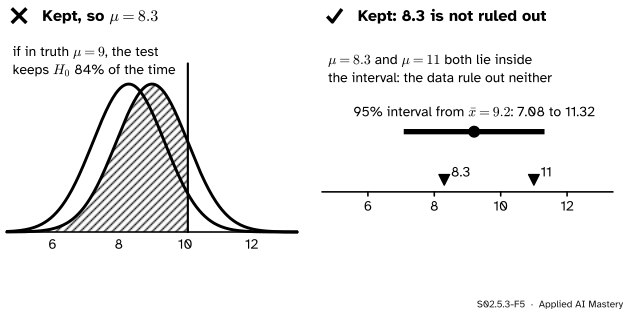
S02.5.3-F5
Wrong beside right. A sample mean of 9.2 keeps \(H_0\), but a test with 25 flats keeps \(H_0\) 84 percent of the time even when the truth is 9. Kept means “not ruled out”, and the interval shows that 11 is not ruled out either.
“We kept \(H_0\), so the site is typical.”
Keeping \(H_0\) means the data are compatible with it, not that it is true. With 25 flats the test would keep \(H_0\) 84 percent of the time even if the site’s mean were 9. The court does not declare the defendant innocent; it says “not proven”. Report what the data allow, for example with the interval of S02.4, as the right panel does and as S02.5.4 explains.
“At level 0.05, a rejection has a 5 percent chance of being wrong.”
\(\alpha\) is \({\Prob(\text{reject} \mid H_0)}\), the false-alarm rate among true nulls. The share of rejections that are wrong is a different conditional probability; in the 1,000-test example of the last lesson it was 47 percent.
“The p-value came out at 0.07, so this time I’ll use \(\alpha = 0.1\).”
Choosing \(\alpha\) after seeing the data removes the guarantee that made it worth choosing. The same mistake in machine learning is picking a classifier’s threshold on the test set: the reported error rates are then too good, because the threshold was fitted to the very examples that score it.
Check yourself
Recall
1. What is a Type I error, and what is its probability in a level-\(\alpha\) test?
Show answer
Rejecting \(H_0\) when it is true. Its probability is \(\alpha\) (at most \(\alpha\) for a count).
2. What is a Type II error, and why is its rate not a single number?
Show answer
Keeping \(H_0\) when it is false. Its rate \(\beta\) depends on which alternative value is true.
3. Write the critical value of the one-sided z-test on the scale of \(\bar{x}\), and its value for the listing site at \({\alpha = 0.05}\).
4. What happens to \(\alpha\) and \(\beta\) when the critical value moves up, with the data fixed?
Show answer
\(\alpha\) falls and \(\beta\) rises: one error is traded for the other.
5. In a classifier, which rates play the parts of \(\alpha\) and \(\beta\)?
Show answer
The false-positive rate (negatives above the threshold) is \(\alpha\); the false-negative rate (positives below it) is \(\beta\).
Exercises
1.★ At \({\alpha = 0.01}\) (one-sided, \({z_{0.99} = 2.326}\)), find the critical value for the listing site. Is \({\bar{x} = 10.5}\) rejected?
Show solution
\({c}\)\({= 8.3 + 2.326 \times 1.082}\)\({= 8.3 + 2.517}\)\({= 10.82}\). Since \({10.5 < 10.82}\) we keep \(H_0\). The p-value 0.021 agrees: it is above 0.01.
2.★★ With \({\alpha = 0.01}\), what is the Type II rate against \({\mu_1 = 11}\)? Compare it with the 0.20 at \({\alpha = 0.05}\).
Show solution
\({(\mu_1 - \mu_0)/\mathrm{SE}}\)\({= 2.7/1.082}\)\({= 2.495}\), so
Cutting the false-alarm rate from 0.05 to 0.01 more than doubles the chance of missing a site whose mean is 11, from 0.20 to 0.43.
3.★★★ Keep \({\alpha = 0.05}\) and the alternative \({\mu_1 = 11}\), but sample 100 flats instead of 25. Find the new critical value and \(\beta\), and explain in terms of the overlap diagram why both errors can now be small at once.
Show solution
\({\mathrm{SE} = 5.41/\sqrt{100} = 0.541}\). The critical value is \({c = 8.3 + 1.645 \times 0.541 = 9.19}\). Then
Four times the data halves the standard error, so both curves become half as wide while their centres stay at 8.3 and 11. They hardly overlap any more, and a single line can leave very little of either curve on the wrong side. The trade between \(\alpha\) and \(\beta\) is forced only for a fixed amount of data.
Summary card
Fix \(\alpha\) first; then two curves and one line show both ways to be wrong.
S02.5.3-F1
Solid: Type I. Hatched: Type II.
Decision. Reject \(H_0\) when the p-value is at most \(\alpha\), fixed before the data.
Errors. Type I rate \(\alpha\); Type II rate \({\beta}\)\({= \Phi(z_{1-\alpha} - (\mu_1 - \mu_0)/\mathrm{SE})}\).
Listing site.\({c = 10.08}\); \({\beta = 0.20}\) against 11; \({\beta = 0.84}\) against 9.
Trade. Moving the line trades \(\alpha\) for \(\beta\), like a classifier’s threshold; more data shrinks both.
Sources and next steps
Sources. Each was opened and checked against this lesson on 15 November 2026.
Jeremy Orloff and Jonathan Bloom, Reading 17b, Null Hypothesis Significance Testing I, MIT OpenCourseWare 18.05 (Spring 2022). Section 4.2 tabulates the two types of error, Section 4.3 defines the significance level as P(reject H0 | H0) and power as P(reject H0 | HA) = 1 minus P(type II error), and Section 7 states the p-test: reject when the p-value is less than the significance level.
David Diez, Mine Cetinkaya-Rundel and Christopher Barr, OpenIntro Statistics, fourth edition (free PDF). Section 5.3.3, decision errors, with the court analogy for Type 1 and Type 2 errors, and Section 5.3.5, choosing a smaller or larger significance level according to the cost of each error.
SciPy developers, scipy.stats.norm: the methods ppf, cdf and sf, with loc and scale for a normal of any mean and spread.