A hypothesis test assumes a dull explanation, works out what data it would produce, and asks how surprising the real data are. Count the exact chance of 7 or more heads in 10 fair tosses, then test a classifier’s 90 of 100 against a baseline of 0.85.
S02.5.1L2 Intermediate25 minIn review (what this means)
The maths and code on this page are checked by automated tests on every change, but an independent reader has not signed it off yet. Spot a mistake or a confusing step? Tell us.
Name the four ingredients of a test: a null hypothesis, an alternative, a test statistic and its distribution if the null hypothesis were true.
Explain a test as proof by contradiction made probabilistic, and say what a small tail does and does not show.
List an exact binomial null distribution with math.comb and compute the tail at least as extreme as an observed count.
Test a classifier’s accuracy against a baseline with scipy.stats.binomtest, choosing the alternative before seeing the data.
The question
A coin lands heads 7 times in 10 tosses. A new classifier answers 90 of 100 test examples correctly, where the model in production manages 85 percent. Each result leans one way. But a fair coin sometimes gives 7 heads, and a model that is no better than 0.85 sometimes gets lucky. How surprised should you be, and how do you put a number on that surprise?
Intuition
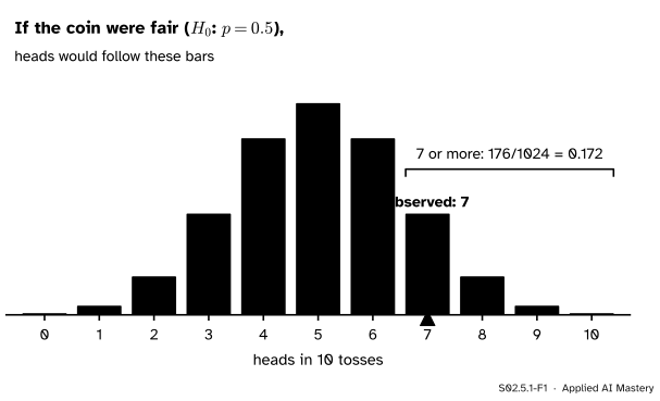
Start from the dullest explanation: the coin is fair. That explanation is precise enough to predict exactly how often each number of heads turns up, so we can look up where 7 falls.
S02.5.1-F1
If the coin were fair, the number of heads would follow these bars. The yellow tail is every result at least as far towards heads as the 7 we saw; together they happen with chance 0.172.
A fair coin gives 7 or more heads about once in every six tries of 10 tosses. That is not rare. Seven heads is no reason to doubt the coin: the dull explanation copes with it easily.
This is the whole logic of a hypothesis test. Assume the dull explanation, work out what data it would produce, and see whether the real data look out of place. If they do, the dull explanation is in trouble. If they do not, it survives, which is not the same as being proved.
Build it up
Step 1. The claim to attack. The null hypothesis\(H_0\) is the dull, precise explanation: here, the chance of heads is \({p = 0.5}\). It must be precise, because we need to compute with it.
Step 2. What we suspect instead. The alternative hypothesis\(H_1\) is what we would believe if \(H_0\) fell. If we only care whether the coin favours heads, \({H_1 : p > 0.5}\), a one-sided alternative. If either direction counts, \({H_1 : p \neq 0.5}\), a two-sided one.
Step 3. One number from the data. The test statistic\(T\) boils the data down to one number that would tend to be large if \(H_1\) were true. For the coin, \(T\) is the number of heads.
Step 4. The world under \(H_0\). The null distribution is the distribution of \(T\) if \(H_0\) were true. Ten independent tosses with chance 0.5 give \({T \sim \mathrm{Bin}(10, 0.5)}\), the binomial family of M06.8.1.
Step 5. Where did we land? Measure how surprising the observed value is by the chance, under \(H_0\), of a value at least as extreme. For \({H_1 : p > 0.5}\), “at least as extreme” means 7 or more.
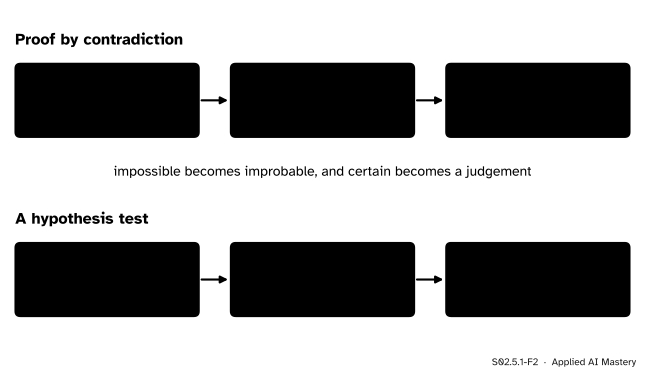
The steps are those of a proof by contradiction, with one change.
S02.5.1-F2
A test borrows the shape of a proof by contradiction. “Impossible” becomes “improbable”, so the conclusion becomes a judgement about how much improbability we will tolerate.
In a proof by contradiction, a single impossible consequence kills the assumption. In a test, nothing is impossible, since a fair coin can give 10 heads. A small tail only says: either \(H_0\) is false, or something unusual happened. The test cannot say which.
The formal statement
NoteThe ingredients of a test
A null hypothesis\(H_0\) that fixes the distribution of the data, such as \({p = p_0}\).
An alternative hypothesis\(H_1\), one-sided (\({p > p_0}\) or \({p < p_0}\)) or two-sided (\({p \neq p_0}\)), chosen before the data are seen.
A test statistic\(T\), computed from the data.
Its null distribution: the distribution of \(T\) when \(H_0\) is true.
For an observed value \(t\) and the one-sided alternative \({p > p_0}\), the evidence against \(H_0\) is the tail \({\Prob(T \ge t \mid H_0)}\). A small tail counts against \(H_0\).
That tail has a name, the p-value, and the next lesson is about it: what it is for two-sided alternatives and for continuous statistics, and what it is not.
For the coin the tail is a finite sum. Under \(H_0\) each of the \({2^{10} = 1024}\) sequences of heads and tails has the same chance, \({1/1024}\), and \({\binom{10}{k}}\) of them have exactly \(k\) heads. So
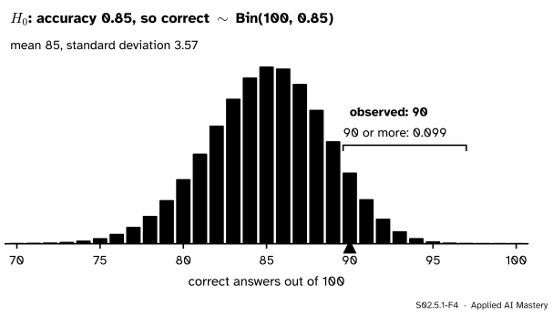
A classifier against a baseline. A model answers 90 of 100 test examples correctly. The production model is right 85 percent of the time, so we ask whether the new one is better. Take \({H_0 : p = 0.85}\), with \(p\) the new model’s accuracy on examples like these, and the one-sided \({H_1 : p > 0.85}\). If the test examples are independent draws, the number correct is \({T \sim \mathrm{Bin}(100, 0.85)}\) under \(H_0\), with mean 85 and standard deviation \({\sqrt{100 \times 0.85 \times 0.15}}\)\({= 3.57}\).
S02.5.1-F4
The null distribution for a model that is right 85 percent of the time on 100 independent examples. Ninety or more correct happens with chance 0.099, about once in ten test sets.
A model no better than the old one would score 90 or more on about one test set in ten. That is weak evidence. Ninety looks clearly better than 85, but 100 examples are too few to tell the two apart with confidence, which is why S02.4 attaches an interval to every test-set score.
Go deeper: why test at the boundary 0.85 when the null is 'no better than 0.85'
The honest null for “is the new model better?” is \({p \le 0.85}\), a whole range of values. We computed the tail only at its edge, \({p = 0.85}\). That is enough, because the tail \({\Prob_p(T \ge 90)}\) grows with \(p\): a worse model is even less likely to reach 90.
To see why, build each example’s outcome from a uniform number \({U_i}\) on \({[0, 1]}\): the model is right when \({U_i < p}\). Raising \(p\) can only turn wrong answers into right ones, never the reverse, so with the same \({U_1, \dots, U_{100}}\) the count \(T\) for a larger \(p\) is never smaller. Every way of reaching 90 at a lower \(p\) also reaches 90 at 0.85. So the boundary gives the largest tail of the whole null range, and a small tail there is small everywhere in it.
Worked example
Is 7 heads in 10 tosses surprising for a fair coin?
Set up.\({H_0 : p = 0.5}\) and \({H_1 : p > 0.5}\), decided before the coin was tossed. The statistic is \({T}\) = the number of heads, and the null distribution is \({\mathrm{Bin}(10, 0.5)}\).
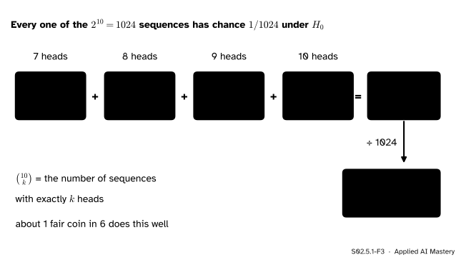
Count the extreme results. “At least as extreme as 7” means 7, 8, 9 or 10 heads. Count the sequences that give each one, with \({\binom{10}{k} = \frac{10!}{k!\,(10-k)!}}\).
S02.5.1-F3
The tail counted by hand: 176 of the 1024 equally likely sequences have 7 or more heads.
\({\binom{10}{9} = 10}\) and \({\binom{10}{10} = 1}\)
Add and divide.\({120 + 45 + 10 + 1 = 176}\) sequences out of 1024, so the tail is \({176/1024 = 0.171875}\), which rounds to 0.172.
Read it. About one fair coin in six would do at least this well. Seven heads gives no good reason to doubt the coin. Had we seen 9 heads, the tail would be \({(10 + 1)/1024 = 0.011}\), about one in a hundred, and doubt would be reasonable.
The classifier, read the same way. Its tail of 0.099 sits between the two: smaller than the coin’s, still about one chance in ten. You would want more test examples before claiming that the new model beats the old one.
Code
First from scratch: list the null distribution with math.comb and add up the tail.
import mathdef binom_pmf(n, p):"""P(T = k) for k = 0, ..., n."""return [math.comb(n, k) * p**k * (1- p)**(n - k) for k inrange(n +1)]ways = [math.comb(10, k) for k inrange(11)]print("sequences with k heads:", ways, " total", sum(ways))tail_ways =sum(ways[7:])coin_tail = tail_ways /2**10print(f"P(T >= 7) = {tail_ways}/1024 = {coin_tail:.6f}")pmf = binom_pmf(100, 0.85)clf_tail =sum(pmf[90:])print(f"classifier: P(T >= 90 | p = 0.85) = {clf_tail:.4f}")print(f"mean {100*0.85:.0f}, standard deviation {math.sqrt(100*0.85*0.15):.2f}")
sequences with k heads: [1, 10, 45, 120, 210, 252, 210, 120, 45, 10, 1]  total 1024
P(T >= 7) = 176/1024 = 0.171875
classifier: P(T >= 90 | p = 0.85) = 0.0994
mean 85, standard deviation 3.57
Then check the logic by simulation: toss 20,000 fair coins ten times each and count how often they reach 7 heads.
import numpy as nprng = np.random.default_rng(0)heads = rng.binomial(10, 0.5, size=20_000)share = np.mean(heads >=7)print(f"share of fair-coin experiments with 7 or more heads: {share:.3f} (exact 0.172)")
share of fair-coin experiments with 7 or more heads: 0.170 (exact 0.172)
Finally the library call. alternative names \(H_1\); 'greater' is the one-sided \({p > p_0}\).
The two numbers match the hand counts. The simulation lands within about 0.01 of the exact tail, as it should with 20,000 tries.
Explore
The module’s interactive, the p-value machine, lives in the next lesson. There you set the number of tosses and the observed count, watch the tail fill in, and run a thousand fair-coin experiments to see how their tails are spread.
Pitfalls
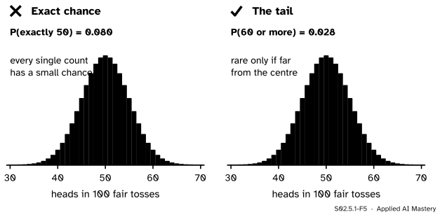
S02.5.1-F5
Wrong beside right. With 100 tosses even the likeliest count, 50, has chance only 0.080, so the chance of the exact result says nothing about surprise. The tail does: 60 or more heads has chance 0.028.
“Seven heads has chance 0.117, so that is what I report.”
The chance of the exact count shrinks as the experiment grows, whatever happens. In 100 fair tosses, getting exactly 50 heads, the most typical result there is, has chance 0.080. Surprise is about how far the result sits from what \(H_0\) expects, so the test adds up everything at least that far: the tail.
“I’ll decide whether to look at heads or tails after I see which one came up more.”
Then the one-sided tail understates the surprise. A coin that came up heavy on either side would have been reported, so both tails belong in the count. Fix \(H_1\) before the data arrive; the next lesson shows that the two-sided tail for the coin is twice the one-sided one, 0.344.
“The tail is 0.172, so there is a 17 percent chance the coin is fair.”
The tail is computed assuming the coin is fair. It is the chance of the data given \(H_0\), not the chance of \(H_0\) given the data. Lesson S02.5.2 shows with counts how far apart the two can be.
Check yourself
Recall
1. Name the four ingredients of a hypothesis test.
Show answer
A null hypothesis \(H_0\), an alternative \(H_1\), a test statistic \(T\), and the null distribution of \(T\): its distribution when \(H_0\) is true.
2. Why must \(H_0\) be precise, such as \({p = 0.5}\), rather than vague?
Show answer
Because the test needs the exact distribution of \(T\) under \(H_0\), and only a precise claim gives one.
3. What is \({\Prob(T \ge 7)}\) for 10 fair tosses, as a fraction and as a decimal?
Show answer
\({176/1024 = 0.172}\).
4. In what way does a test differ from a proof by contradiction?
Show answer
A proof derives something impossible; a test derives only something improbable. A small tail means either \(H_0\) is false or something unusual happened, and the test cannot say which.
5. A classifier gets 90 of 100 right. What tail does the one-sided test against accuracy 0.85 give, and what does it suggest?
Show answer
\({\Prob(T \ge 90) = 0.099}\) under \({p = 0.85}\): a model no better than the baseline would do this on about one test set in ten, so the evidence of improvement is weak.
Exercises
1.★ A coin gives 9 heads in 10 tosses. Find the one-sided tail \({\Prob(T \ge 9)}\) under \({p = 0.5}\) by counting sequences.
Show solution
Nine heads: \({\binom{10}{9} = 10}\) sequences. Ten heads: 1 sequence. So the tail is \({11/1024 = 0.0107}\), about one fair coin in a hundred. In code: the pvalue of stats.binomtest(9, 10, 0.5, alternative="greater") is 0.0107.
2.★★ On a small test set of 20 examples a model answers 19 correctly. The baseline accuracy is 0.75. Set up the one-sided test and compute the tail by hand.
Show solution
\({H_0 : p = 0.75}\), \({H_1 : p > 0.75}\), \({T \sim \mathrm{Bin}(20, 0.75)}\) under \(H_0\). The results at least as extreme are 19 and 20:
A model no better than 0.75 scores 19 or 20 out of 20 about once in 41 test sets: much stronger evidence than the classifier’s 90 of 100, even though 95 percent and 90 percent look similar.
3.★★★ Show that for \({T \sim \mathrm{Bin}(n, p)}\) and any fixed \(t\), the tail \({\Prob_p(T \ge t)}\) never decreases as \(p\) increases, and explain why this lets us test “\({p \le 0.85}\)” at the single value 0.85.
Show solution
Let \({U_1, \dots, U_n}\) be independent and uniform on \({[0, 1]}\) and set \({T_p}\) = the number of \(i\) with \({U_i < p}\). Each event \({U_i < p}\) has chance \(p\) and the events are independent, so \({T_p \sim \mathrm{Bin}(n, p)}\). If \({p < p'}\), then \({U_i < p}\) implies \({U_i < p'}\), so \({T_p \le T_{p'}}\) for every outcome. Hence the event \({T_p \ge t}\) is contained in \({T_{p'} \ge t}\), and
\[
\Prob(T_p \ge t) \le \Prob(T_{p'} \ge t).
\]
For the null range \({p \le 0.85}\) the largest tail is therefore at \({p = 0.85}\). If the tail is small there, it is small for every \(p\) in the null range, so testing at the boundary is the cautious choice.
Summary card
Assume the dull explanation, and ask how surprising the data would be.
S02.5.1-F1
The tail at least as extreme as 7 heads.
Ingredients.\(H_0\), \(H_1\) (one- or two-sided, fixed in advance), a statistic \(T\), its null distribution.
Evidence. The tail \({\Prob(T \ge t \mid H_0)}\): small counts against \(H_0\).
Coin.\({176/1024 = 0.172}\). Classifier. 90 of 100 against 0.85 gives 0.099.
Library.stats.binomtest(k, n, p, alternative="greater"), then its pvalue.
Sources and next steps
Sources. Each was opened and checked against this lesson on 15 November 2026.
David Diez, Mine Cetinkaya-Rundel and Christopher Barr, OpenIntro Statistics, fourth edition (free PDF). Section 5.3.1, the hypothesis testing framework: the null and alternative hypotheses, the null value, and the court analogy in which failing to convict is not a finding of innocence.
Jeremy Orloff and Jonathan Bloom, Reading 17b, Null Hypothesis Significance Testing I, MIT OpenCourseWare 18.05 (Spring 2022). Section 3.1 lists the ingredients (null and alternative hypotheses, test statistic, null distribution, rejection region), and Example 3 in Section 4 tests a coin flipped 10 times with the null distribution Bin(10, 0.5).
SciPy developers, scipy.stats.binomtest: the signature binomtest(k, n, p=0.5, alternative='two-sided'), the alternatives 'two-sided', 'greater' and 'less', and the result’s pvalue.
Next.S02.5.2 The p-value names the tail, extends it to two-sided alternatives and to the z-test, and proves that under \(H_0\) it is spread evenly between 0 and 1.