Build confidence intervals for a difference of two means (pooled and Welch) and of two proportions from one rule, variances add, then turn the margin formula round to find how many observations or test examples a target precision needs.
S02.4.4L2 Intermediate25 minIn review (what this means)
The maths and code on this page are checked by automated tests on every change, but an independent reader has not signed it off yet. Spot a mistake or a confusing step? Tell us.
Derive the standard error of a difference of two independent means from Var(X - Y) = Var(X) + Var(Y).
Compute pooled and Welch t-intervals for a difference of means, with the Welch degrees of freedom, by hand and with scipy.stats.ttest_ind.
Compute an interval for the difference of two proportions and use it to compare two models tested on separate test sets.
Choose the sample size for a target margin, for a mean and for a proportion, and explain why it grows with the square of the precision.
The question
Five visitors shown design B stayed 10 minutes on average; five shown design A stayed 7. Two models scored 0.90 and 0.87 on separate test sets of 1,000. Are these differences real, or noise? And if you want a model’s accuracy to within 2 points, how many test examples must you label?
From the last lesson
1. Why does the Wald interval fail for 10 correct out of 10?
Show answer
Its standard error \({\sqrt{\hat{p}(1 - \hat{p})/n}}\) is zero at \(\hat{p} = 1\), so the interval is the single point 1. Wilson gives 0.722 to 1.
2. What are the Wilson and Clopper-Pearson intervals for 90 correct of 100?
Show answer
Wilson 0.826 to 0.945; Clopper-Pearson 0.824 to 0.951.
Intuition
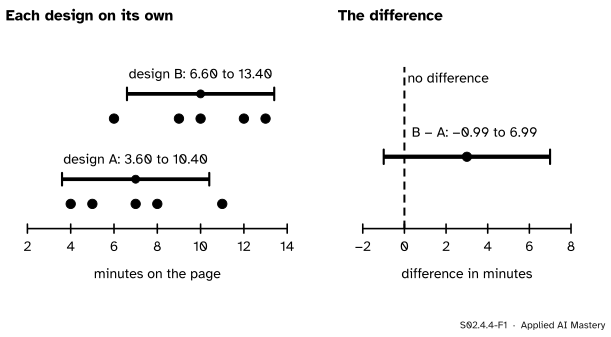
To compare two groups, build one interval for the difference rather than one interval for each group. The two separate intervals answer “where is each mean?”; only the interval for the difference answers “how far apart are they?”.
The difference of two sample means wobbles more than either mean alone, because both wobble. But it wobbles less than the two wobbles added end to end, because they are independent and partly cancel.
S02.4.4-F1
Left: each design’s own 95 percent t-interval. Right: the one interval that answers the question, for the difference of means B minus A: \(-0.99\) to \(6.99\) minutes. It contains 0, so five visitors per design cannot tell us which design holds visitors longer.
The interval for the difference is centred on \(10 - 7 = 3\) minutes and is wide: the data fit design B being a minute worse or seven minutes better. That is an honest summary of ten visitors.
Build it up
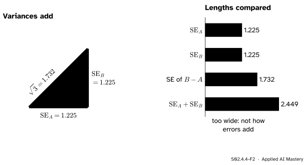
Step 1. Variances add. For any two random variables, \({\mathrm{Var}(X - Y)} = {\mathrm{Var}(X)} + {\mathrm{Var}(Y)} - {2\,\mathrm{Cov}(X, Y)}\) (M06.10). If the two samples are independent, the covariance is zero and
Step 2. Standard errors combine like the sides of a right triangle. Taking square roots, the standard error of the difference is \({\sqrt{\mathrm{SE}_A^2 + \mathrm{SE}_B^2}}\), the hypotenuse of a triangle whose legs are the two standard errors.
S02.4.4-F2
For design A and design B each estimated standard error is \({\sqrt{7.5/5}} = 1.225\). The standard error of the difference is \({\sqrt{1.5 + 1.5}} = {\sqrt{3}} = 1.732\), longer than either leg but shorter than their sum.
Step 3. Estimate the variances. Two ways are common. The pooled method assumes the two populations share one variance and estimates it from both samples at once. The Welch method lets them differ and estimates each separately. Both then use a \(t\) multiplier.
Step 4. The same for proportions. Two accuracies \(\hat{p}_1\) and \(\hat{p}_2\) from independent test sets have variances \({p_1(1-p_1)/n_1}\) and \({p_2(1-p_2)/n_2}\), and these add in the same way.
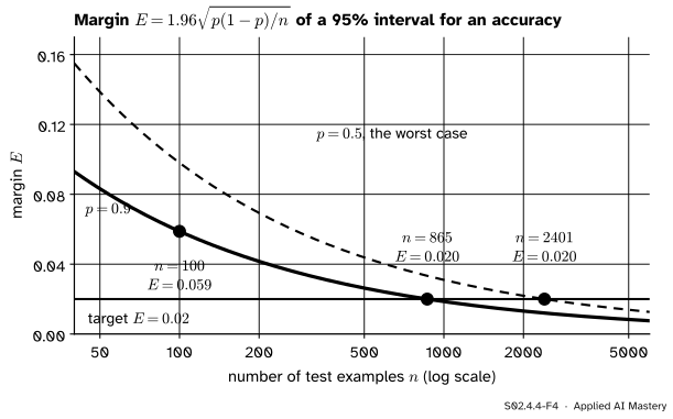
Step 5. Turn the margin round. A margin is a multiplier times a standard error, and the standard error shrinks like \({1 / \sqrt{n}}\). Fix the margin you want and solve for \(n\).
S02.4.4-F4
The margin of a 95 percent interval for an accuracy, against the number of test examples. To halve the margin you need four times the examples.
The formal statement
NoteIntervals for a difference
Two independent samples of sizes \(n_A\) and \(n_B\), means \(\bar{x}_A, \bar{x}_B\) and variances \(s_A^2, s_B^2\). The 95 percent interval for \(\mu_B - \mu_A\) is \({(\bar{x}_B - \bar{x}_A)} \pm {t_{\nu,\,0.975}\,\widehat{\mathrm{se}}}\), with:
Welch:\(\widehat{\mathrm{se}} = {\sqrt{s_A^2/n_A + s_B^2/n_B}}\) and \(\nu\) from the Welch-Satterthwaite formula below.
For two proportions from independent samples, the Wald-type interval is \({(\hat{p}_1 - \hat{p}_2)} \pm {1.96\,\widehat{\mathrm{se}}}\), where \(\widehat{\mathrm{se}}^2\) is \({\hat{p}_1(1-\hat{p}_1)/n_1} + {\hat{p}_2(1-\hat{p}_2)/n_2}\).
The pooled variance weights each sample’s variance by its degrees of freedom:
It is usually not a whole number. It lies between the smaller of \(n_A - 1, n_B - 1\) and \(n_A + n_B - 2\), and equals the pooled \(\nu\) when the sizes and the variances are equal. Welch is the safer default. When the variances really are equal it still covers about 95 percent and is only a little wider (about 4 percent for five observations per group, in a simulation of normal data). When they are not and the sample sizes differ, the pooled interval can cover far less: five observations with standard deviation 3 against twenty with standard deviation 1 give the pooled interval a simulated coverage of about 73 percent, and Welch about 95.
Sample size for a margin. For a mean with standard deviation \(\sigma\), the margin of a 95 percent interval is \(E = {z_{0.975}\,\sigma / \sqrt{n}}\). Solve for \(n\): multiply both sides by \({\sqrt{n}}\), divide by \(E\), and square:
\[
\sqrt{n} = \frac{z_{0.975}\,\sigma}{E} ,
\]
\[
n = \Bigl(\frac{z_{0.975}\,\sigma}{E}\Bigr)^2 .
\]
For a proportion, \(\sigma^2 = {p(1 - p)}\), so \(n = {z_{0.975}^2\,p(1-p) / E^2}\). Round up, never down: a smaller \(n\) gives a wider margin than you asked for. If you have no idea of \(p\), use \(p = 0.5\), where \({p(1-p)}\) is largest.
Worked example
Design B minus design A. Both samples have five visitors and \(s^2 = 7.5\).
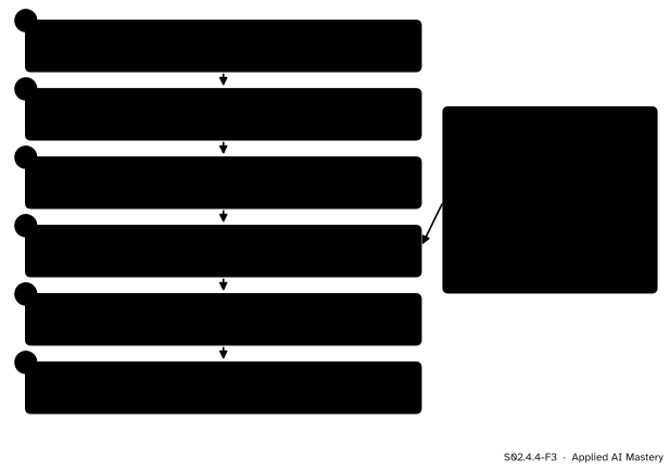
S02.4.4-F3
The pooled two-sample t-interval for design B minus design A, with the Welch check.
Multiplier.\(\nu = 8\), and \({t_{8,\,0.975}} = 2.306\).
Interval.\({3 \pm 2.306 \times 1.732 = 3 \pm 3.99}\): from \(-0.99\) to \(6.99\).
Welch. Here \(a = b = {7.5 / 5} = 1.5\), so the standard error is again \({\sqrt{3}}\) and \(\nu = {3^2 / (1.5^2/4 + 1.5^2/4)} = {9 / 1.125} = 8\). Welch gives the same interval because the sizes and variances are equal.
Two models on separate test sets. Model 1 gets 900 of 1,000 right and model 2 gets 870 of a different 1,000. The variances of the two accuracies are \({0.9 \times 0.1 / 1000} = 0.00009\) and \({0.87 \times 0.13 / 1000} = 0.000113\); they add to \(0.000203\), whose square root is \(0.01425\). The interval is \({0.03 \pm 1.96 \times 0.01425 = 0.03 \pm 0.028}\): 0.002 to 0.058. It just excludes 0.
Sample sizes. To pin an accuracy near 0.9 to within 2 points: \({1.96^2 \times 0.09 / 0.02^2 = 864.4}\), so 865 examples. With no idea of the accuracy, \(p = 0.5\) gives \({1.96^2 \times 0.25 / 0.0004} = 2400.9\), so 2,401. For the mean rent of the city to within 1 (one hundred euros) at 95 percent, \({(1.96 \times 5.41 / 1)^2} = 112.4\), so 113 flats.
Code
From scratch, both versions of the two-sample interval.
import mathimport numpy as npfrom scipy import statsa = np.array([4, 5, 7, 8, 11], dtype=float) # design Ab = np.array([6, 9, 10, 12, 13], dtype=float) # design Bdef two_sample(x, y, pooled=True, level=0.95):"""Interval for mean(y) - mean(x), with its degrees of freedom.""" nx, ny =len(x), len(y) vx, vy = x.var(ddof=1), y.var(ddof=1)if pooled: sp2 = ((nx -1) * vx + (ny -1) * vy) / (nx + ny -2) se, nu = math.sqrt(sp2 * (1/ nx +1/ ny)), nx + ny -2else: u, v = vx / nx, vy / ny se, nu = math.sqrt(u + v), (u + v) **2/ (u**2/ (nx -1) + v**2/ (ny -1)) q = stats.t.ppf(0.5+ level /2, nu) d = y.mean() - x.mean()return d - q * se, d + q * se, se, nufor pooled in (True, False): lo, hi, se, nu = two_sample(a, b, pooled)print("pooled"if pooled else"Welch ", f"se {se:.3f} nu {nu:.2f} interval {lo:.2f} to {hi:.2f}")
pooled se 1.732  nu 8.00  interval -0.99 to 6.99
Welch  se 1.732  nu 8.00  interval -0.99 to 6.99
SciPy’s ttest_ind returns a result whose confidence_interval() is the interval for the first sample’s mean minus the second’s, so put design B first. equal_var=False asks for Welch.
for equal_var in (True, False): res = stats.ttest_ind(b, a, equal_var=equal_var) ci = res.confidence_interval(confidence_level=0.95)print(f"equal_var={equal_var}: df {res.df:.1f} interval {ci.low:.2f} to {ci.high:.2f}")
equal_var=True:  df 8.0  interval -0.99 to 6.99
equal_var=False:  df 8.0  interval -0.99 to 6.99
Why Welch is the safer default, by simulation on normal data with a true difference of 0: equal spreads and sizes, then a small noisy group beside a large quiet one.
rng = np.random.default_rng(1)def pooled_and_welch(na, nb, sd_a, sd_b, reps=20_000):"""Coverage of the pooled and Welch intervals, and Welch's mean width over pooled's.""" x, y = rng.normal(0, sd_a, (reps, na)), rng.normal(0, sd_b, (reps, nb)) d = y.mean(axis=1) - x.mean(axis=1) va, vb = x.var(axis=1, ddof=1), y.var(axis=1, ddof=1) sp2 = ((na -1) * va + (nb -1) * vb) / (na + nb -2) half_p = stats.t.ppf(0.975, na + nb -2) * np.sqrt(sp2 * (1/ na +1/ nb)) u, v = va / na, vb / nb nu = (u + v) **2/ (u**2/ (na -1) + v**2/ (nb -1)) half_w = stats.t.ppf(0.975, nu) * np.sqrt(u + v)return (np.mean(np.abs(d) <= half_p), np.mean(np.abs(d) <= half_w), half_w.mean() / half_p.mean())equal = pooled_and_welch(5, 5, 1, 1)unequal = pooled_and_welch(5, 20, 3, 1)print("5 and 5, sd 1 and 1: pooled %.3f Welch %.3f width ratio %.3f"% equal)print("5 and 20, sd 3 and 1: pooled %.3f Welch %.3f width ratio %.3f"% unequal)
5 and 5, sd 1 and 1:  pooled 0.950  Welch 0.956  width ratio 1.037
5 and 20, sd 3 and 1: pooled 0.731  Welch 0.946  width ratio 2.230
Then the two models and the sample sizes, rounding up with math.ceil.
z = stats.norm.ppf(0.975)p1, p2, n =0.90, 0.87, 1000se_d = math.sqrt(p1 * (1- p1) / n + p2 * (1- p2) / n)print(f"difference {p1 - p2:.2f}, se {se_d:.5f}, interval {p1 - p2 - z * se_d:.3f} to {p1 - p2 + z * se_d:.3f}")for name, p in (("model 1", p1), ("model 2", p2)): half = z * math.sqrt(p * (1- p) / n)print(f"{name} alone: {p - half:.3f} to {p + half:.3f}")sigma =5.409395527800759# the city's standard deviationprint("accuracy near 0.9, E = 0.02:", math.ceil(z**2*0.09/0.02**2))print("no idea of p, E = 0.02:", math.ceil(z**2*0.25/0.02**2))print("city mean rent, E = 1: ", math.ceil((z * sigma /1) **2))
difference 0.03, se 0.01425, interval 0.002 to 0.058
model 1 alone: 0.881 to 0.919
model 2 alone: 0.849 to 0.891
accuracy near 0.9, E = 0.02: 865
no idea of p,      E = 0.02: 2401
city mean rent,    E = 1:    113
With \(z = 1.96\) exactly, \({1.96^2 \times 0.09 / 0.0004} = 864.36\); with \(z = 1.95996\) it is 864.33. Either way, 865.
Explore
The module’s interactive, the dance of confidence intervals, lives in lesson S02.4.1. Use it to feel the square-root law behind sample-size planning: note the average width at \(n = 25\), then at \(n = 100\). The width roughly halves.
Pitfalls
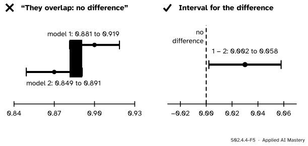
S02.4.4-F5
Left: the two models’ own intervals overlap. Right: yet the interval for their difference excludes zero.
“Their intervals overlap, so the difference is not real.”
Overlap is the wrong test. Separate intervals add the two margins end to end (0.0186 + 0.0208 = 0.039 here), but the difference’s margin is the hypotenuse, 0.028. Two 95 percent intervals can overlap while the interval for the difference excludes zero, as here. Always build the interval for the difference.
“Both models were scored on the same 1,000 examples, so I use the two-sample interval.”
The two-sample interval needs independent samples. On a shared test set the two models’ errors are correlated (both find the same examples hard), the covariance term no longer vanishes, and the right analysis is paired: look at the differences example by example. That is lesson S02.7.1, with McNemar’s test in S02.7.2.
“864.4 examples, so 864 will do.”
Rounding down gives a margin a little wider than the target. Always round a sample size up. And remember the square: halving the margin needs four times the data, so a margin of 1 point near 0.9 needs about 3,458 examples, not 1,730.
Check yourself
Recall
1. Why is the standard error of a difference of independent means the square root of a sum?
Show answer
Because \({\mathrm{Var}(X - Y)} = {\mathrm{Var}(X)} + {\mathrm{Var}(Y)}\) when the covariance is zero, so the variances add, and the standard error is the square root of that sum.
2. Give the 95 percent interval for design B minus design A.
Show answer
\(3 \pm {2.306 \times \sqrt{3}} = 3 \pm 3.99\), from \(-0.99\) to \(6.99\) minutes.
3. When do the pooled and Welch intervals agree exactly?
Show answer
When the two samples have the same size and the same variance; then the standard errors match and the Welch degrees of freedom equal \(n_A + n_B - 2\).
4. How many test examples pin an accuracy near 0.9 to within 2 points at 95 percent?
Show answer
\({1.96^2 \times 0.09 / 0.02^2} = 864.4\), rounded up to 865.
5. Two 95 percent intervals overlap. Can the difference still be clearly non-zero?
Show answer
Yes. The two models with 900 and 870 correct of 1,000 have overlapping intervals, but the interval for the difference is 0.002 to 0.058.
Exercises
1.★ How many flats must be sampled for a 95 percent interval of half-width 0.5 for the city’s mean rent (\(\sigma = 5.41\))?
Show solution
\(n = {(1.96 \times 5.41 / 0.5)^2} = {(21.21)^2} = 449.7\), so 450 flats. Halving the margin from 1 to 0.5 multiplies the 113 flats by about four.
2.★★ Design A (five visitors, mean 7, \(s^2 = 7.5\)) is compared with a design C seen by ten visitors, mean 9, \(s^2 = 2\). Compute the Welch interval for C minus A.
Show solution
\(a = {7.5 / 5} = 1.5\) and \(b = {2 / 10} = 0.2\), so \(\widehat{\mathrm{se}} = {\sqrt{1.7}} = 1.304\). The degrees of freedom are
Then \({t_{5.10,\,0.975}} = 2.556\), the margin is \({2.556 \times 1.304 = 3.33}\), and the interval is \(2 \pm 3.33\), from \(-1.33\) to \(5.33\). The small, noisy design A dominates the standard error, and Welch’s \(\nu\) of about 5 reflects that it carries most of the uncertainty.
3.★★★ You can show a total of \(N\) visitors either design, with the same \(\sigma\) in both groups. Show that splitting them equally gives the narrowest interval for the difference.
Show solution
With \(n_A = m\) and \(n_B = N - m\), the variance of the difference is \({f(m)} = {\sigma^2\,(1/m + 1/(N - m))}\). Its derivative is
which is zero when \(m^2 = {(N - m)^2}\), that is \(m = N/2\). The second derivative, \({\sigma^2\,(2/m^3 + 2/(N - m)^3)}\), is positive, so this is a minimum. At the equal split the variance is \({4\sigma^2 / N}\).
Summary card
Compare with one interval for the difference, and plan \(n\) from the margin you need.
Barbara Illowsky and Susan Dean, Introductory Statistics 2e, OpenStax, Section 8.1 (\(n = {z^2\sigma^2 / \mathrm{EBM}^2}\), always rounded up) and Section 8.3 (\(n = {z^2 p'q' / \mathrm{EBP}^2}\), with \(p' = 0.5\) when nothing is known).
scipy.stats.ttest_ind, SciPy reference: equal_var=False performs Welch’s test, and the result’s confidence_interval(confidence_level=0.95) is an interval for the difference in population means.
David Diez, Mine Cetinkaya-Rundel and Christopher Barr, OpenIntro Statistics, 4th edition: Section 6.2 on the difference of two proportions and Section 7.3 on the difference of two means.
Next. Module S02.5, Hypothesis tests and p-values, turns an interval into a decision: a two-sided test rejects a value exactly when it lies outside the interval. S02.6 plans sample sizes for tests rather than margins, and S02.7 handles paired designs.