Put an honest interval around a classifier’s test accuracy. See by exact calculation why the textbook Wald interval falls short near 0 and 1, derive the Wilson interval by solving a quadratic, and meet the exact Clopper-Pearson interval.
S02.4.3L2 Intermediate25 minIn review (what this means)
The maths and code on this page are checked by automated tests on every change, but an independent reader has not signed it off yet. Spot a mistake or a confusing step? Tell us.
Compute the Wald interval for a proportion and explain why it plugs the estimate into the standard error.
Compute the exact coverage of an interval for a count by adding binomial probabilities over all outcomes.
Derive the Wilson interval by solving a quadratic inequality in p, and compute it for 90 correct of 100.
Report a model’s test accuracy with a Wilson or Clopper-Pearson interval using scipy.stats.binomtest.
The question
A classifier gets 90 of 100 test examples right, and the report says “accuracy 0.90”. The next test set of 100 could easily give 0.86 or 0.94. What range of true accuracies do these 100 answers actually support, and does the formula in most textbooks keep its 95 percent promise here?
From the last lesson
1. What is the 95 percent t-interval for design A’s times, 4, 5, 7, 8 and 11?
Show answer
\(7 \pm {2.776 \times 1.225} = 7 \pm 3.40\), from 3.60 to 10.40 minutes.
2. Why does “1.96 with \(s\)” cover too rarely for small normal samples?
Show answer
Because \(s\) is itself random, \({(\bar{X} - \mu) / (S / \sqrt{n})}\) follows \(t_{n-1}\), whose tails are heavier than the normal’s. For \(n = 5\), 1.96 with \(s\) covers about 88 percent of the time.
Intuition
Accuracy is a proportion: score each test example 1 if the model gets it right and 0 if not, and the accuracy \(\hat{p}\) is the mean of those scores. So the machinery of S02.4.1 applies: the central limit theorem makes \(\hat{p}\) roughly normal around the true accuracy \(p\), with standard error \({\sqrt{p(1 - p)/n}}\) (S02.1.2). The textbook Wald interval plugs \(\hat{p}\) in for the unknown \(p\) and takes plus or minus 1.96 of those.
For a count we can do better than simulate. Every possible outcome, 0 to 100 correct, has a binomial probability, so the coverage of any interval can be added up exactly, for every true \(p\).
S02.4.3-F1
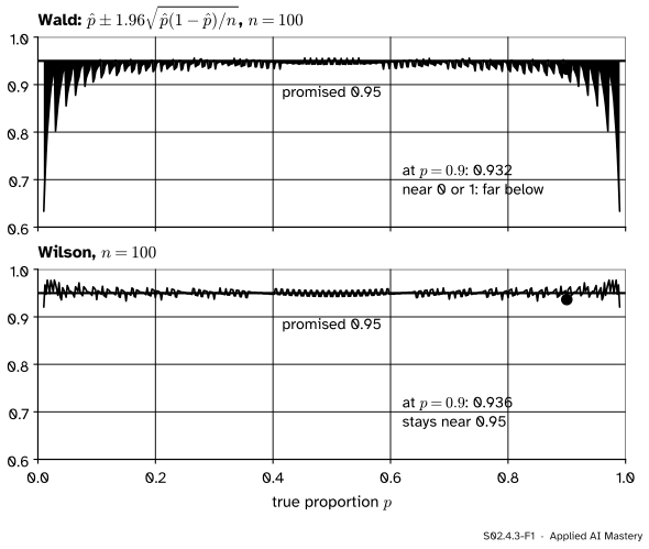
Exact coverage of 95 percent intervals for \(n = 100\) test examples. Top: the Wald interval falls short almost everywhere and badly near 0 and 1. Bottom: the Wilson interval stays close to the promise. The sawtooth comes from the count being a whole number.
The Wald interval fails where machine learning lives: good classifiers have accuracies near 1, and rare events have rates near 0. The Wilson interval fixes this with one change, derived below: it never puts the guess \(\hat{p}\) inside the standard error.
Build it up
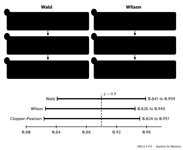
Step 1. The Wald interval for 90 of 100. The estimate is \(\hat{p} = 0.9\). Its estimated standard error is \({\sqrt{0.9 \times 0.1 / 100}} = {\sqrt{0.0009}} = 0.03\), so the interval is \({0.9 \pm 1.96 \times 0.03}\), which is \({0.9 \pm 0.059}\): 0.841 to 0.959.
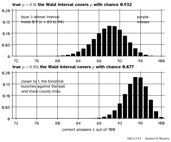
Step 2. Coverage, counted exactly. Fix a true accuracy, say \(p = 0.9\). For each possible count \(k\), compute the Wald interval from \({k / 100}\) and ask whether it contains 0.9. The coverage is the total binomial probability of the counts that answer yes.
S02.4.3-F2
Coverage of the Wald interval, counted outcome by outcome. Blue counts give intervals that hold the true \(p\); purple counts give misses.
Step 3. See why it misses. At \(p = 0.95\) the counts 98, 99 and 100 are likely, but their intervals are tiny: \(\hat{p} = 1\) gives standard error \({\sqrt{1 \times 0 / 100}} = 0\) and the “interval” 1 to 1. The plug-in standard error is smallest exactly where the estimate is most extreme, so the interval is most overconfident where it is most wrong.
Step 4. Keep \(p\) in the standard error. Ask instead: which values of \(p\) are within 1.96 of their own standard errors of the observed \(\hat{p}\)? That is a condition on \(p\) alone, and the next section solves it.
The formal statement
NoteThree intervals for a proportion
With \(k\) successes in \(n\) independent trials, \(\hat{p} = {k / n}\) and \(z = z_{0.975} = 1.96\):
Wilson: every \(p\) with \({\abs{\hat{p} - p}} \le {z\sqrt{p(1 - p)/n}}\). Its ends are given below.
Clopper-Pearson (exact): every \(p\) for which the observed \(k\) is not in either 2.5 percent tail of the binomial distribution. Its coverage is at least 0.95 for every \(p\).
Deriving the Wilson interval. Both sides of the condition are non-negative, so squaring keeps it equivalent:
The left side is a parabola in \(p\) that opens upwards, so it is at most zero exactly between its two roots. The quadratic formula gives them; inside the square root,
because the \(4\hat{p}^2\) terms cancel and what is left is \({4\hat{p}z^2/n} + {z^4/n^2} - {4\hat{p}^2z^2/n}\). The square root of that is \(2z\) times \({\sqrt{\hat{p}(1-\hat{p})/n + z^2/(4n^2)}}\). Putting it into the quadratic formula and dividing top and bottom by 2 gives the Wilson interval, a centre plus or minus a half-width:
Two features explain why it behaves. Its centre, \({(k + z^2/2) / (n + z^2)}\), is \(\hat{p}\) pulled a little towards one half, as if we had added about two successes and two failures. And its half-width never shrinks to zero: even at \(\hat{p} = 1\) the term \({z^2 / (4n^2)}\) keeps it open.
S02.4.3-F3
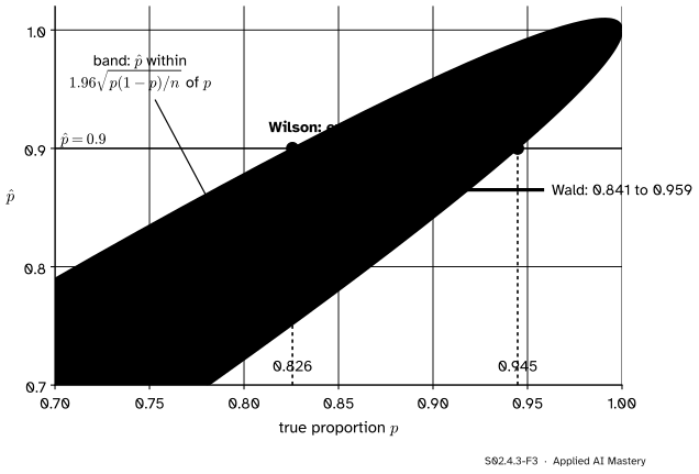
The Wilson interval read off a picture. For each true \(p\) (across), the band holds the estimates within 1.96 of their standard errors. The Wilson interval for \(\hat{p} = 0.9\) is where the horizontal line at 0.9 sits inside the band. The Wald interval (grey) is shifted towards 1.
Go deeper: where the Clopper-Pearson interval comes from
The exact interval inverts two one-sided binomial tests. Its lower end is the \(p\) at which seeing \(k\) or more successes has probability exactly 0.025, and its upper end is the \(p\) at which seeing \(k\) or fewer has probability 0.025. Those ends are quantiles of beta distributions: \({\mathrm{Beta}(k, n - k + 1)}\) at 0.025 and \({\mathrm{Beta}(k + 1, n - k)}\) at 0.975. Because the count is discrete, it cannot hit 0.95 exactly, and it errs on the safe side: its coverage is at least 0.95 everywhere (0.956 at \(p = 0.9\) for \(n = 100\)), so it is a little wider than it needs to be on average. Brown, Cai and DasGupta recommend Wilson (or the Jeffreys interval) for small \(n\).
The roots of \({1.038415\,p^2} - {1.838415\,p} + 0.81 = 0\) are 0.826 and 0.945. The centre is \({(90 + 1.92) / (100 + 3.84)} = 0.885\), a little below 0.9.
Clopper-Pearson. From the beta quantiles: 0.824 to 0.951, slightly wider than Wilson, as the interval with guaranteed coverage usually is.
All three agree that a true accuracy anywhere from about 0.83 to 0.95 fits these 100 answers. A report of “accuracy 0.90” alone hides a range twelve points wide.
Code
From scratch: the two formulas and an exact coverage function that adds binomial probabilities with math.comb.
import mathdef wald(k, n, z=1.959964): p = k / n half = z * math.sqrt(p * (1- p) / n)return p - half, p + halfdef wilson(k, n, z=1.959964): p = k / n centre = (p + z**2/ (2* n)) / (1+ z**2/ n) half = z / (1+ z**2/ n) * math.sqrt(p * (1- p) / n + z**2/ (4* n**2))return centre - half, centre + halfdef coverage(method, n, p):"""Exact: the total binomial probability of the counts whose interval holds p.""" total =0.0for k inrange(n +1): lo, hi = method(k, n)if lo <= p <= hi: total += math.comb(n, k) * p**k * (1- p) ** (n - k)return totalprint("Wald 90/100:", [round(v, 3) for v in wald(90, 100)])print("Wilson 90/100:", [round(v, 3) for v in wilson(90, 100)])for n, p in ((100, 0.9), (100, 0.95), (100, 0.99), (10, 0.9)):print(f"n={n:3d} p={p}: Wald {coverage(wald, n, p):.3f} Wilson {coverage(wilson, n, p):.3f}")
Wald  90/100: [0.841, 0.959]
Wilson 90/100: [0.826, 0.945]
n=100 p=0.9:  Wald 0.932   Wilson 0.936
n=100 p=0.95:  Wald 0.877   Wilson 0.966
n=100 p=0.99:  Wald 0.633   Wilson 0.921
n= 10 p=0.9:  Wald 0.650   Wilson 0.930
At \(p = 0.9\) the two are close, both a little under 0.95 because of the sawtooth. Nearer the wall Wald drops to 0.877 and then 0.633, while Wilson stays between 0.92 and 0.97. With only ten test examples, Wald covers 65 percent of the time.
Now the library. scipy.stats.binomtest returns a result whose proportion_ci method offers 'wilson' and 'exact' (Clopper-Pearson, the default).
from scipy import statsresult = stats.binomtest(90, 100)for method in ("wilson", "exact"): ci = result.proportion_ci(confidence_level=0.95, method=method)print(f"{method:7s}{ci.low:.3f} to {ci.high:.3f}")
wilson  0.826 to 0.945
exact   0.824 to 0.951
Explore
The module’s interactive lives in lesson S02.4.1. Switch it to a proportion, set the true accuracy to 0.95 and \(n\) to 20, and add a few hundred intervals with the Wald method, then with Wilson. The running coverage tells the story of the anchor figure in a minute.
Pitfalls
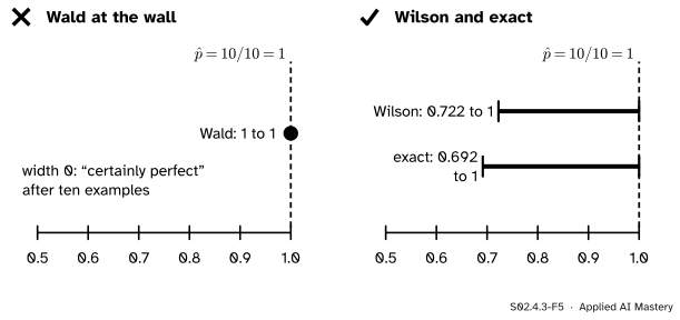
S02.4.3-F5
Ten right out of ten. Left: the Wald interval has zero width. Right: Wilson and the exact interval admit true accuracies as low as about 0.7.
“Ten out of ten: the interval is 1 to 1, so the model is perfect.”
The Wald interval’s standard error is zero when \(\hat{p}\) is 0 or 1, so it claims certainty from ten examples. Wilson gives 0.722 to 1 and Clopper-Pearson 0.692 to 1. Small test sets for rare classes hit this wall all the time.
“With 100 examples the normal approximation is fine.”
It depends on \(p\) as well as \(n\). At \(n = 100\) the Wald interval covers 0.932 at \(p = 0.9\), 0.877 at \(p = 0.95\) and 0.633 at \(p = 0.99\). Use Wilson by default; it costs nothing.
“The test set was used to pick the model, and its accuracy has a 95 percent interval.”
The interval assumes the test examples are a fresh random sample and the model was fixed before looking. If the test set chose among many models, the best score is biased upwards and its interval is too optimistic (S02.9 and ML01.9).
Check yourself
Recall
1. Why is accuracy on a test set a proportion?
Show answer
It is the mean of 0/1 scores, one per test example: the share of examples the model gets right.
2. Write the Wald interval and give it for 90 correct of 100.
Show answer
\(\hat{p} \pm {1.96\sqrt{\hat{p}(1 - \hat{p})/n}}\); for 90 of 100, \(0.9 \pm 0.059\), from 0.841 to 0.959.
3. How is the exact coverage of an interval for a count computed?
Show answer
For a fixed true \(p\), add the binomial probabilities of all counts \(k\) whose interval contains \(p\).
4. What inequality does the Wilson interval solve for \(p\)?
Show answer
\({\abs{\hat{p} - p}} \le {1.96\sqrt{p(1 - p)/n}}\): the standard error uses the candidate \(p\), not \(\hat{p}\). Squaring gives a quadratic in \(p\), and the interval is between its roots.
5. Give the Wilson and Clopper-Pearson intervals for 90 correct of 100.
Show answer
Wilson 0.826 to 0.945; Clopper-Pearson 0.824 to 0.951.
Exercises
1.★ A model gets 45 of 50 right. Give the Wald interval and compare it with 90 of 100.
Show solution
\(\hat{p} = 0.9\) and \(\widehat{\mathrm{se}} = {\sqrt{0.09 / 50}} = 0.0424\). The margin is \({1.96 \times 0.0424 = 0.083}\), so the interval is 0.817 to 0.983. Same accuracy, half the examples, and the margin is \({\sqrt{2}} = 1.41\) times as wide.
2.★★ A spam filter makes no mistakes on 20 test emails. Use the Wilson formula with \(\hat{p} = 0\) to find the upper end of a 95 percent interval for its error rate.
Show solution
With \(\hat{p} = 0\) the formula’s centre is \({(z^2 / (2n)) / (1 + z^2/n)}\) and its half-width is \({(z / (1 + z^2/n))\cdot z / (2n)}\), which is the same number. So the lower end is 0 and the upper end is twice the centre:
The two weights are positive and add to one. For \(n = 100\) the weight on \(\hat{p}\) is \({100 / 103.84} = 0.963\) and the weight on one half is 0.037, so for \(\hat{p} = 0.9\) the centre is \({0.963 \times 0.9 + 0.037 \times 0.5 = 0.885}\). The pull fades as \(n\) grows.
Summary card
Do not put the guess in the standard error: solve for every \(p\) the data allow.
S02.4.3-F1
Wald sags at the walls; Wilson holds.
Wald.\(\hat{p} \pm {1.96\sqrt{\hat{p}(1-\hat{p})/n}}\): 0.841 to 0.959 for 90 of 100.
Wilson. Roots of \({\abs{\hat{p} - p}} = {1.96\sqrt{p(1-p)/n}}\): 0.826 to 0.945.
Clopper-Pearson. Exact, at least 95 percent coverage: 0.824 to 0.951.
Sources. Each was opened and checked against this lesson on 15 November 2026.
Lawrence D. Brown, T. Tony Cai and Anirban DasGupta, Interval estimation for a binomial proportion, Statistical Science 16(2), 101 to 133, 2001 (the abstract, on the Astrostatistics and Astroinformatics Portal). The coverage of the standard Wald interval is erratic, the problem is far more persistent than is appreciated, and the authors recommend the Wilson interval or the equal-tailed Jeffreys interval for small \(n\).
Jeremy Orloff and Jonathan Bloom, Reading 23b: Confidence intervals for the mean of non-normal data, MIT OpenCourseWare 18.05, Spring 2022. Section 3 builds conservative normal intervals for a Bernoulli proportion from the central limit theorem and the bound \(\sigma \le 1/2\).
BinomTestResult.proportion_ci, SciPy reference: the methods 'exact' (Clopper-Pearson, the default), 'wilson' and 'wilsoncc', citing Clopper and Pearson (1934) and Wilson (1927).