Turn the sampling distribution of the mean round into a range for the unknown mean, watch a hundred such ranges dance around the truth, and learn exactly what the 95 percent does and does not promise.
S02.4.1L2 Intermediate25 minIn review (what this means)
The maths and code on this page are checked by automated tests on every change, but an independent reader has not signed it off yet. Spot a mistake or a confusing step? Tell us.
Derive the z-interval for a mean by turning a probability statement about the sample mean into one about the population mean.
Compute a 95 percent z-interval by hand and with scipy.stats.norm.interval.
Explain the 95 percent as the share of intervals, over repeated samples, that cover the true mean, and check it by simulation.
Predict how the width changes with the sample size and with the confidence level.
Name and correct the common misreadings of a single computed interval.
The question
You draw 25 flats from the city and their rents average 8.77 hundred euros a month. A report says “the mean rent is 8.77, with a 95 percent confidence interval from 6.65 to 10.89”. What exactly is 95 percent sure here, and of what?
Intuition
A sample mean is a guess at the population mean \(\ctruth{\mu}\), and S02.1 showed that the guess wobbles from sample to sample with a known spread, the standard error. A confidence interval replaces the single guess with a range: the sample mean plus or minus a margin, chosen so that the range catches \(\ctruth{\mu}\) for most samples.
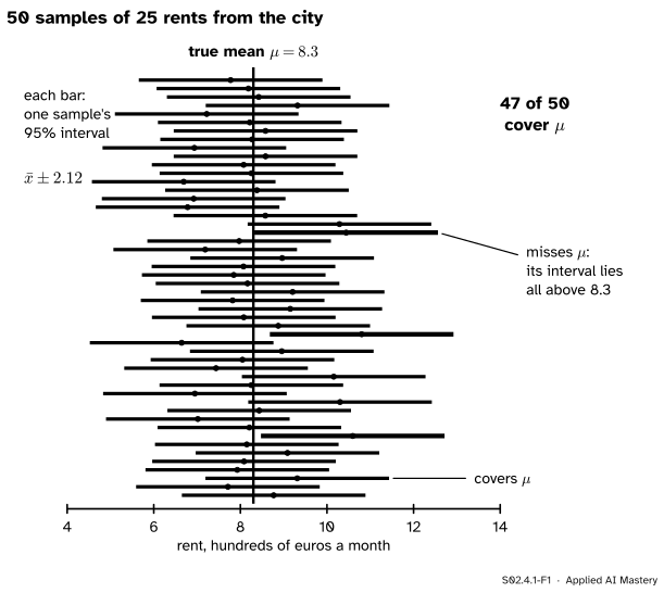
The city of S01 lets us watch this happen, because it is invented and we know its true mean, \(\mu = 8.3\). Draw 25 rents, build the range, then do it again, fifty times.
S02.4.1-F1
The dance of confidence intervals. Each bar is one sample of 25 rents and its interval \({\bar{x} \pm 2.12}\). The bars move from sample to sample; the true mean stays put. Here 47 of 50 cover \(\mu\); the three misses are drawn in the loss colour.
The picture holds the whole idea. The intervals are random: each new sample moves its bar. The truth is fixed: the black line never moves. “95 percent” describes the bars as a crowd: in the long run, 95 of every 100 bars made this way cross the line. It says nothing about a chance that the line jumps into one particular bar.
This is the same promise a test-set score needs. A model’s accuracy on 100 test examples is one draw from a sampling distribution, and an interval around it says how far the true accuracy could plausibly be. Lesson S02.4.3 builds that interval.
Build it up
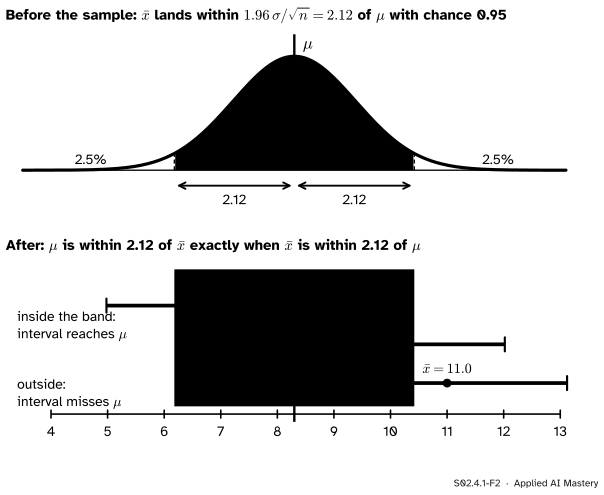
Step 1. Where the sample mean lands. By the central limit theorem (M06.11.3), for \(n = 25\) the sample mean \(\bar{X}\) is close to normal, centred on \(\mu\), with standard error \({\sigma / \sqrt{n}} = {5.41 / 5} = 1.082\). A normal variable lies within 1.96 standard deviations of its centre with chance 0.95, so before we draw, \(\bar{X}\) has a 95 percent chance of landing within \({1.96 \times 1.082 = 2.12}\) of \(\mu\).
Step 2. Turn the statement round. “The sample mean is within 2.12 of \(\mu\)” and “\(\mu\) is within 2.12 of the sample mean” are the same statement: both say the distance between the two numbers is at most 2.12. So the range \({\bar{X} \pm 2.12}\) catches \(\mu\) exactly when \(\bar{X}\) lands in the middle band of the top curve below.
S02.4.1-F2
The pivot. Top: before sampling, \(\bar{X}\) lands within 2.12 of \(\mu\) with chance 0.95. Bottom: a sample mean inside that band gives an interval that reaches \(\mu\); one outside gives an interval that misses. So the intervals cover \(\mu\) exactly as often as the means land in the band.
Step 3. Count the hits. The chance that the interval covers \(\mu\) is therefore the chance that \(\bar{X}\) lands in the band: 0.95. In the anchor figure 47 of 50 landed there; over 10,000 samples in the code below the share is 0.951.
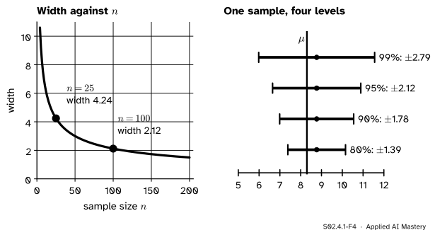
Step 4. What sets the width. The interval is \(\bar{x}\) plus or minus \({z \times \sigma / \sqrt{n}}\), so three things set its width: the spread \(\sigma\) of the population, the sample size \(n\), and the multiplier \(z\), which comes from the confidence level you choose.
S02.4.1-F4
Left: the width falls like \({1 / \sqrt{n}}\), so four times the data halves it (4.24 at \(n = 25\), 2.12 at \(n = 100\)). Right: for one sample, a higher confidence level buys a wider interval.
The formal statement
NoteDefinition: confidence interval
An interval \([L, U]\) whose ends are computed from the sample is a \(1 - \alpha\) confidence interval for a parameter \(\theta\) if, whatever the true value of \(\theta\),
\[
\Prob(L \le \theta \le U) = 1 - \alpha .
\]
The probability is over repeated samples: \(L\) and \(U\) are random, \(\theta\) is not. The number \(1 - \alpha\) (0.95 for \(\alpha = 0.05\)) is the confidence level, and the share of intervals that actually cover \(\theta\) is the coverage. An interval whose coverage is only close to \(1 - \alpha\) is called approximate.
The z-interval. Suppose the data are \(n\) independent draws from a population with mean \(\mu\) and a known standard deviation \(\sigma\), and write \(\mathrm{SE} = {\sigma / \sqrt{n}}\). Capital \(\bar{X}\) is the sample mean before we draw (a random variable); small \(\bar{x}\) is the number we get. The derivation has four lines.
First, the standardised mean is a pivot: a quantity that involves \(\mu\) but whose distribution does not depend on \(\mu\). By the central limit theorem, approximately,
\[
Z = \frac{\bar{X} - \mu}{\mathrm{SE}} \sim N(0, 1).
\]
Second, the middle 95 percent of \({N(0, 1)}\) runs from \(-z_{0.975}\) to \(z_{0.975} = 1.96\), so the following event has probability 0.95:
Third, multiply all three parts of the inequality by the positive number \(\mathrm{SE}\); the inequalities keep their direction, so this is the same event:
Each step rewrote one event without changing it, so its probability is still 0.95. Only the last form has \(\mu\) alone in the middle, and it is a confidence interval:
For any level \(1 - \alpha\), replace \(z_{0.975}\) by \({z_{1 - \alpha/2}}\): 1.645 for 90 percent and 2.576 for 99 percent.
Go deeper: when the 95 percent is exact, and when it is approximate
If the population itself is normal, \(\bar{X}\) is exactly normal for every \(n\) and the z-interval covers \(\mu\) with probability exactly 0.95. The city is skewed to the right, so for the city the first line holds only approximately, by the central limit theorem, and the coverage is only close to 0.95. The simulation in the code checks how close: 0.951 at \(n = 25\). The misses are lopsided, though: a sample that happens to hold a few Centre penthouses drags \(\bar{x}\) high, so intervals that lie wholly above \(\mu\) are more common than intervals that lie wholly below it.
Knowing \(\sigma\) but not \(\mu\) is rare outside an invented city. Lesson S02.4.2 replaces \(\sigma\) by the sample’s own \(s\) and pays for it with a larger multiplier.
Worked example
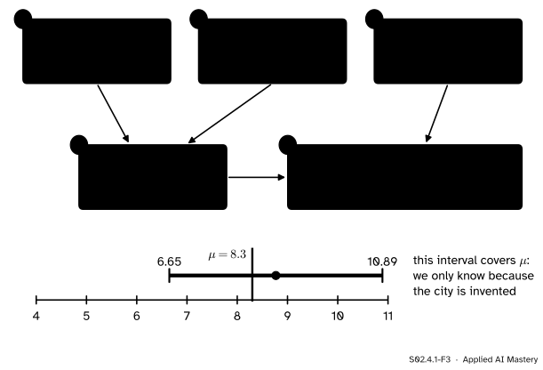
The 25 rents of the hook. One sample of 25 flats, drawn with replacement from the city, has mean \(\bar{x} = 8.77\). The city’s \(\sigma = 5.41\) is known.
S02.4.1-F3
The worked example as a trace: three ingredients, the margin, then the interval.
So the 95 percent interval is 6.65 to 10.89. The true mean 8.3 is inside it, but only the invented city lets us check that. With real data we never learn whether our interval is one of the 95 hits or one of the 5 misses.
The other levels. The same sample gives 90 percent: \({8.77 \pm 1.645 \times 1.082}\), which is \({8.77 \pm 1.78}\), from 6.99 to 10.55. And 99 percent: \({8.77 \pm 2.576 \times 1.082}\), which is \({8.77 \pm 2.79}\), from 5.98 to 11.56. More confidence, wider range, the same data.
Code
First the city, built exactly as in S01, and the interval from scratch. The standard library’s NormalDist gives the quantile, so nothing is hidden.
import mathfrom statistics import NormalDistimport numpy as nprng = np.random.default_rng(0)parts = []for mean, size in ((5, 250), (8, 150), (17, 100)): draws = rng.gamma(9.0, 1.0, size) parts.append(draws * mean / draws.mean())rents = np.concatenate(parts)mu, sigma = rents.mean(), rents.std() # the truth, known only because the city is inventeddef z_interval(sample, sigma, level=0.95): z = NormalDist().inv_cdf(0.5+ level /2) # 1.96 for 95 percent half = z * sigma / math.sqrt(len(sample)) centre =sum(sample) /len(sample)return centre - half, centre + halfrng = np.random.default_rng(0)samples = rng.choice(rents, (100, 25)) # 100 samples of 25 rents, i.i.d. drawsintervals = [z_interval(s, sigma) for s in samples]covers = [lo <= mu <= hi for lo, hi in intervals]print("mu =", round(mu, 2), " sigma =", round(sigma, 2))print("first interval:", [round(v, 2) for v in intervals[0]])print("cover mu: first 50:", sum(covers[:50]), " all 100:", sum(covers))
mu = 8.3  sigma = 5.41
first interval: [np.float64(6.65), np.float64(10.89)]
cover mu: first 50: 47   all 100: 94
One hundred intervals is a small crowd. Ten thousand show the long-run share, and which side the misses fall on.
Finally the library call. scipy.stats.norm.interval returns the middle share of a normal distribution; centred on \(\bar{x}\) with scale \({\sigma / \sqrt{n}}\), that is the z-interval.
from scipy import statsxbar = samples[0].mean()for level in (0.80, 0.90, 0.95, 0.99): lo, hi = stats.norm.interval(level, loc=xbar, scale=sigma /5)print(f"{level:.0%}: {lo:.2f} to {hi:.2f} half-width {(hi - lo) /2:.2f}")
80%: 7.38 to 10.16   half-width 1.39
90%: 6.99 to 10.55   half-width 1.78
95%: 6.65 to 10.89   half-width 2.12
99%: 5.98 to 11.56   half-width 2.79
The simulated coverage, 0.951, is within simulation error of 0.95 (with 10,000 samples the share itself wobbles by about 0.002). The misses are not shared evenly: about 3.5 percent of intervals lie wholly above \(\mu\) and 1.4 percent wholly below, the skew of the city showing through.
Explore
S02.4-X1
The dance of confidence intervals
Draw samples one at a time or a hundred at once and watch the running coverage settle near the promised level. Change \(n\) and the level to see the width move, then switch to a proportion and compare the Wald and Wilson methods at a true accuracy near 1.
Things to try. Choose the z method, set the level to 80 percent and add a few hundred intervals: about one in five misses. Then set \(n = 5\) and choose the t method: the coverage of the skewed city falls short of the promise, which is the subject of the next lesson.
Pitfalls
S02.4.1-F5
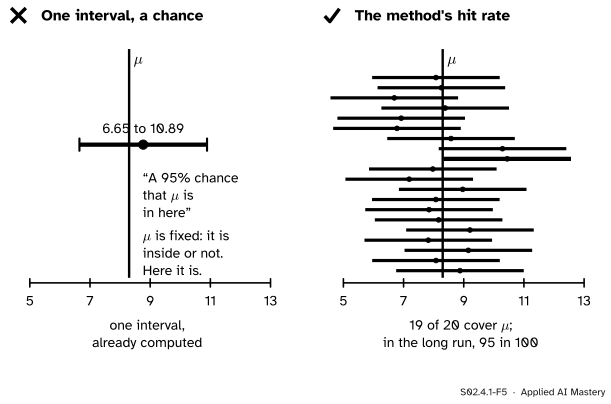
Left: once computed, an interval either holds \(\mu\) or it does not. Right: the 95 percent is the hit rate of the method over many samples.
“There is a 95 percent chance that \(\mu\) lies between 6.65 and 10.89.”
Before sampling, the interval is random and has a 95 percent chance of covering \(\mu\). After sampling, both 6.65, 10.89 and \(\mu\) are fixed numbers, so the statement is simply true or false (here true, as only the invented city can tell us). Say instead: “the interval was made by a method that covers the true mean in 95 percent of samples”. A probability for \(\mu\) itself needs a prior, which is the Bayesian route of S04.
“95 percent of the rents lie between 6.65 and 10.89.”
The interval is about the mean, not about single flats. Only 26 percent of the city’s 500 rents lie in that range, because single rents spread with \(\sigma = 5.41\) while the mean of 25 spreads with \({\sigma / 5}\). In machine learning the same slip confuses the uncertainty of an average error with the spread of individual errors.
“The misses fall evenly on both sides.”
Only when the sampling distribution is symmetric. For the right-skewed city, 3.5 percent of intervals lie wholly above \(\mu\) and 1.4 percent wholly below. The total is right, the split is not, which matters when only one side of the error is costly.
Check yourself
Recall
1. In the dance of intervals, which part is random and which is fixed?
Show answer
The intervals are random: each sample moves its interval. The true mean \(\mu\) is fixed.
2. Write the 95 percent z-interval for a mean.
Show answer
\(\bar{x} \pm {1.96\,\sigma / \sqrt{n}}\), with \(\sigma\) the known population standard deviation.
3. What is a pivot, and which pivot gives the z-interval?
Show answer
A quantity that involves the parameter but whose distribution does not depend on it. Here \({(\bar{X} - \mu) / (\sigma / \sqrt{n})}\), which is (approximately) \({N(0, 1)}\) whatever \(\mu\) is.
4. How does the width change if the sample size is multiplied by four?
Show answer
It halves, because the width is proportional to \({1 / \sqrt{n}}\) and \({\sqrt{4}} = 2\).
5. A 95 percent interval came out as 6.65 to 10.89. Is there a 95 percent chance that \(\mu\) is in it?
Show answer
No. After the sample is drawn, \(\mu\) is either in it or not. The 95 percent is the share of intervals from this method that cover \(\mu\) over repeated samples.
Exercises
1.★ A population has known \(\sigma = 12\). A sample of 36 has mean 50. Give the 95 and the 99 percent z-intervals.
Show solution
The standard error is \({12 / \sqrt{36}} = {12 / 6} = 2\). For 95 percent the margin is \({1.96 \times 2 = 3.92}\), so the interval is 46.08 to 53.92. For 99 percent the margin is \({2.576 \times 2 = 5.152}\), so the interval is 44.85 to 55.15 (to two decimals).
2.★★ You run the z-interval method 200 times on independent samples. How many intervals do you expect to miss \(\mu\), and what is the chance that none of them does?
Show solution
Each interval misses with probability 0.05, independently, so the number of misses is binomial with \(n = 200\) and \(p = 0.05\). Its mean is \({200 \times 0.05 = 10}\). The chance of no miss at all is \({0.95^{200}}\), which is about \({3.5 \times 10^{-5}}\). A report of 200 intervals that all cover the truth should make you suspicious, not reassured.
3.★★★ Show that the 95 percent z-interval is the shortest interval of the form \({[\bar{x} - a\,\mathrm{SE},\; \bar{x} + b\,\mathrm{SE}]}\) with coverage 0.95 when the pivot is exactly normal.
Show solution
Coverage 0.95 means \({\Phi(a)} - {\Phi(-b)} = 0.95\), where \(\Phi\) is the standard normal distribution function, and the width is \({(a + b)\,\mathrm{SE}}\). Hold the coverage fixed: differentiating the constraint gives \({\varphi(a)\,da} + {\varphi(b)\,db} = 0\), where \(\varphi\) is the normal density, so \({db / da} = {-\varphi(a) / \varphi(b)}\). The width changes at the rate
which is zero only when \({\varphi(a)} = {\varphi(b)}\), that is \(a = b\) (both are positive and \(\varphi\) falls on \([0, \infty)\)). If \(a < b\) then \({\varphi(a)} > {\varphi(b)}\) and the rate is negative, so raising \(a\) shortens the interval; if \(a > b\) the rate is positive. The width is therefore smallest at \(a = b\), and then \({2\Phi(a)} - 1 = 0.95\) gives \(a = 1.96\).
Summary card
The interval moves; the truth stays put; 95 percent of the intervals catch it.
S02.4.1-F1
Fifty samples, fifty intervals, 47 hits.
Pivot.\({(\bar{X} - \mu) / (\sigma / \sqrt{n})}\) is about \({N(0, 1)}\), whatever \(\mu\) is.
Width. Proportional to \(\sigma\), to \(z\), and to \({1 / \sqrt{n}}\).
Meaning. 95 percent is the coverage of the method, not a chance for one interval.
Sources and next steps
Sources. Each was opened and checked against this lesson on 15 November 2026.
Jeremy Orloff and Jonathan Bloom, Reading 22: Confidence intervals based on normal data, MIT OpenCourseWare 18.05, Spring 2022. Section 4.1 defines the z confidence interval for normal data with known variance, writing its multiplier as the right critical value \({z_{\alpha/2}}\) (our \({z_{1-\alpha/2}}\)), Sections 4.3 and 4.4 obtain it by pivoting, and Section 3 warns that the confidence level is never a probability that the parameter lies in the interval computed from the given data.
Jeremy Orloff and Jonathan Bloom, Reading 23a: Confidence intervals, three views, MIT OpenCourseWare 18.05, Spring 2022. Section 5 gives the formal definition (the interval contains the true value with probability \(1 - \alpha\) for every possible value) and Section 7 explains why the level is not the probability that one computed interval holds the mean.
Barbara Illowsky and Susan Dean, Introductory Statistics 2e, Section 8.1, OpenStax: the interval for a mean with known \(\sigma\), and its reading that 95 percent of all intervals constructed this way contain the true mean.