With a mean and a spread to estimate, the likelihood becomes a hill over a plane. Climb it for five visitors’ times: both partial derivatives vanish at the sample mean and at the variance with divisor n, the Hessian confirms a peak, and the same steps turn a line with normal noise into least squares.
S02.3.3L2 Intermediate30 minIn review (what this means)
The maths and code on this page are checked by automated tests on every change, but an independent reader has not signed it off yet. Spot a mistake or a confusing step? Tell us.
Write the log-likelihood of a normal sample as a function of the mean and the standard deviation, and read it as a surface and as contours.
Derive the maximum likelihood estimates of the mean and variance by setting both partial derivatives to zero, and confirm a peak with the Hessian.
Explain why the MLE of the variance divides by n, and compute it beside s squared for a small sample.
Show that, for a line with independent normal noise, maximum likelihood gives the least-squares line.
The question
Five visitors shown page design A (invented) spent 4, 5, 7, 8 and 11 minutes on it. If these are draws from a normal distribution, which mean and which spread fit them best? Now there are two dials to turn at once, so the likelihood is no longer a curve but a hill over a plane. Climbing it answers a second question too: why is squared error the standard loss for regression?
From the last lesson
1. What is the MLE of an exponential rate, and what is it for the waiting times 1, 3, 0.5, 2.5, 3?
Show answer
\({\hat{\lambda} = 1/\bar{x}}\), which is \({1/2 = 0.5}\) per minute for the waiting times.
2. Why did the derivative not find the MLE of the upper end of a uniform?
Show answer
Where the likelihood is positive it is \({\theta^{-n}}\), which only falls, so its derivative is never zero. The top is at the edge of the allowed values, the largest observation.
Intuition
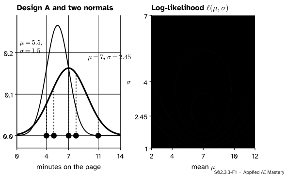
Each pair of a mean \(\mu\) and a standard deviation \(\sigma\) is a normal curve. Its likelihood is the product of the curve’s heights at the five times. Plot that score at every point of the \({(\mu, \sigma)}\) plane and you get a landscape with one hill.
S02.3.3-F1
Left: design A’s five times and two candidate normal curves. The thick one, \({\mu = 7}\) and \({\sigma = 2.45}\), gives the data the largest product of heights. Right: the log-likelihood over every \({(\mu, \sigma)}\), as contours. The peak is the MLE; the thin curve’s pair sits several rings down.
A narrow curve is tall, but only near its centre: the thin curve at \({(5.5, 1.5)}\) gives the times 8 and 11 almost no height, and the product collapses. A very wide curve reaches every time but is low everywhere. The hill’s top balances centre and spread.
Build it up
Step 1. One observation. The normal density at \(x\) is
The data enter only through the sum of squared deviations from \(\mu\). That sum is a loss in disguise, and it is the term the climb has to make small.
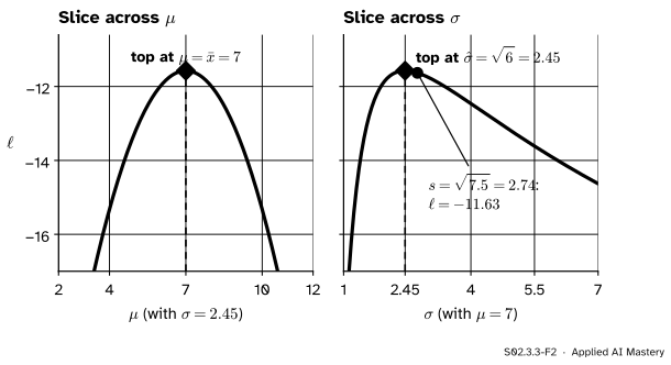
Step 4. Slices. Fix \(\sigma\) and walk across \(\mu\): only the sum of squares changes, so the slice is an upside-down parabola with its top at the \(\mu\) that makes the sum smallest, the mean (S01.3.1). Fix \({\mu = 7}\) and walk across \(\sigma\): the first term pulls \(\sigma\) down, the last pushes it up, and they balance at one value.
S02.3.3-F2
Two slices through the hill. Across \(\mu\) the top is at \({\bar{x} = 7}\) whatever \(\sigma\) is. Across \(\sigma\) the top is at \({\sqrt{6} = 2.45}\), a little left of \({s = \sqrt{7.5} = 2.74}\).
The formal statement
NoteResult: the normal MLE
For independent observations \({x_1, \dots, x_n}\) from \({N(\mu, \sigma^2)}\) with \({n \ge 2}\), not all equal, the log-likelihood has a single peak at
The MLE of the variance divides by \(n\), not by \({n - 1}\).
Derivation. Take the partial derivative of \(\ell\) with respect to each parameter, holding the other fixed (M05.2). The first two terms of \(\ell\) have no \(\mu\) in them, and \({\pd{}{\mu}(x_i - \mu)^2 = -2(x_i - \mu)}\), so
It is zero when \({\sum x_i = n\mu}\), so \({\hat{\mu} = \bar{x}}\), whatever \(\sigma\) is. With respect to \(\sigma\), using \({\tfrac{d}{d\sigma}\sigma^{-2} = -2\sigma^{-3}}\),
Set it to zero, multiply by \({\sigma^3 / n}\) and put \({\mu = \bar{x}}\): \({\hat{\sigma}^2 = \tfrac{1}{n}\sum (x_i - \bar{x})^2}\). By invariance (S02.3.2), the MLE of \(\sigma^2\) is the square of the MLE of \(\sigma\), so it does not matter which of the two we treat as the parameter.
It is a peak. The second partial derivatives (M05.5) are
At the peak \({\sum (x_i - \bar{x}) = 0}\) and \({\sum (x_i - \bar{x})^2 = n\hat{\sigma}^2}\), so the mixed entry vanishes and the last entry is \({n/\hat{\sigma}^2 - 3n/\hat{\sigma}^2 = -2n/\hat{\sigma}^2}\). The Hessian there is
with both diagonal entries negative and no off-diagonal part: negative definite, so the flat point is a maximum. It is also the top of the whole hill. For any \(\sigma\), moving \(\mu\) to \(\bar{x}\) makes the sum of squares smaller, so it raises \(\ell\). Along \({\mu = \bar{x}}\), \({\pd{\ell}{\sigma} = (n\hat{\sigma}^2 - n\sigma^2)/\sigma^3}\) is positive below \(\hat{\sigma}\) and negative above it, so that slice climbs to \(\hat{\sigma}\) and then falls.
S02.3.3-F4
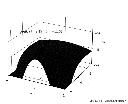
The same log-likelihood as a surface. One hill, steep on the side of small \(\sigma\), where a narrow curve misses the data badly, and gentle on the side of large \(\sigma\). Values below \(-20\) are cut off flat.
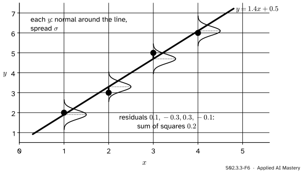
Least squares is maximum likelihood. Now let the mean depend on an input: the model of a line with normal noise says that \({y_i = w x_i + b + \varepsilon_i}\), with the errors \(\varepsilon_i\) independent and \({N(0, \sigma^2)}\). Then \(y_i\) is normal with mean \({w x_i + b}\), and Step 3 with \(\mu\) replaced by \({w x_i + b}\) gives
For any fixed \(\sigma\), the parameters \(w\) and \(b\) appear only in the sum of squared residuals, with a minus sign. So the \(w\) and \(b\) that maximise the likelihood are exactly those that minimise the sum of squares: the least-squares line of ML01.4.2. Then the \(\sigma\) step goes through as before, giving \({\hat{\sigma}^2 = \tfrac{1}{n}\sum \closs{(y_i - \hat{y}_i)^2}}\).
S02.3.3-F6
The four points of ML01.4 under the model “normal around the line”. Each point’s density is largest when its residual is small, and the log-likelihood charges each residual by its square: the least-squares line \({y = 1.4x + 0.5}\) is the maximum likelihood line.
Worked example
Fit a normal to design A’s times 4, 5, 7, 8, 11.
S02.3.3-F3
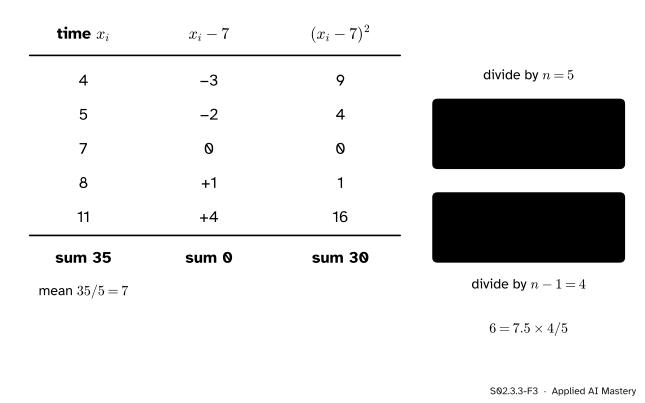
The deviations from the mean, their squares, and the two divisors.
Mean.\({\hat{\mu} = 35/5 = 7}\) minutes.
Squared deviations. 9, 4, 0, 1, 16, adding to 30.
MLE of the variance.\({\hat{\sigma}^2 = 30/5 = 6}\), so \({\hat{\sigma} = \sqrt{6} = 2.449}\). The sample variance of S01.3.3 is \({s^2 = 30/4 = 7.5}\): the MLE is \({4/5}\) of it.
Height of the peak. Put \({\sum (x_i - 7)^2 = n\hat{\sigma}^2}\) into \(\ell\):
Hessian.\({-n/\hat{\sigma}^2 = -5/6 = -0.833}\) and \({-2n/\hat{\sigma}^2 = -10/6 = -1.667}\), both negative, so a peak.
The line. For the four points of ML01.4 the least-squares line is \({y = 1.4x + 0.5}\) with residuals 0.1, \(-0.3\), 0.3, \(-0.1\). Their squares add to 0.2, so \({\hat{\sigma}^2 = 0.2/4 = 0.05}\).
Code
From scratch: the formulas, then a grid search over the plane to confirm that nothing beats them.
The library: scipy.stats.norm.fit maximises the likelihood and returns the location and the scale, \({\hat{\mu}}\) and \({\hat{\sigma}}\). For the line, maximising \(\ell\) numerically over \(w\), \(b\) and \(\ln\sigma\) (the log keeps \(\sigma\) positive) lands on the least-squares answer of np.polyfit.
from scipy import optimize, statsloc, scale = stats.norm.fit(a)print("norm.fit:", loc, round(scale**2, 6))x = np.array([1, 2, 3, 4.0])y = np.array([2, 3, 5, 6.0])def neg_ell(params): w, b, log_sigma = params sigma = np.exp(log_sigma) residuals = y - (w * x + b) # each y_i is normal around w x_i + breturnlen(y) * np.log(sigma) +len(y) /2* np.log(2* np.pi) + np.sum(residuals**2) / (2* sigma**2)fit = optimize.minimize(neg_ell, x0=[0.0, 0.0, 0.0])w_ml, b_ml, sigma2_ml = fit.x[0], fit.x[1], np.exp(2* fit.x[2])print("maximum likelihood:", np.round([w_ml, b_ml, sigma2_ml], 4), " polyfit:", np.round(np.polyfit(x, y, 1), 4))
The negative log-likelihood of the line is the normal one with each \(\mu\) replaced by \({w x_i + b}\): the residuals enter only through their sum of squares, as the derivation said.
Explore
S02.3-X1
Likelihood surface explorer
Drag a data point along the line, or choose it and use its slider, and watch the peak move. Add points up to eight, fix \(\mu\) with the slider to see the slice through the hill, and compare the MLE of \(\sigma^2\) with \(s^2\) in the read-out.
Three things to try. Drag the 11 out to 15: the peak moves right by \({4/5 = 0.8}\) and up, because one far point raises both the mean and the spread. Pull all five points close together: the hill becomes narrow and tall. Then add three points: with \({n = 8}\) the ratio \({\hat{\sigma}^2 / s^2}\) is \({7/8}\), closer to 1 than \({4/5}\).
Pitfalls
S02.3.3-F5
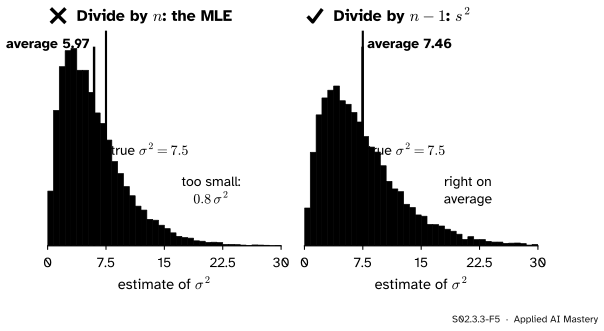
Wrong beside right, in a seeded simulation of samples of five. The MLE of the variance averages about 6.0, four fifths of the true 7.5; \(s^2\) averages about 7.5.
“Maximum likelihood is the best method, so the variance should divide by \(n\).”
The MLE divides by \(n\) because it measures spread around \(\bar{x}\), the point that the same data chose to be as close as possible. By S02.2.1 it is biased low, with average \({\tfrac{n-1}{n}\sigma^2}\): 0.8 times the truth for \({n = 5}\). For small samples, report \(s^2\); for large ones the two agree.
“The MLE of \(\sigma\) is the square root of \(s^2\).”
The MLE of \(\sigma\) is \({\sqrt{\hat{\sigma}^2} = \sqrt{6} = 2.45}\) for design A, not \({s = \sqrt{7.5} = 2.74}\). Invariance connects \(\hat{\sigma}\) to \(\hat{\sigma}^2\), not to \(s^2\).
“Least squares is always the right loss for regression.”
It is the maximum likelihood loss when the errors are independent, normal and of equal spread. If the errors have heavier tails, a few large ones dominate the sum of squares. Under Laplace errors, for example, the likelihood charges each residual by its absolute value instead, and the best constant is the median rather than the mean. Choosing a loss is choosing a noise model.
Check yourself
Recall
1. What are the MLEs of \(\mu\) and \(\sigma^2\) for a normal sample?
Show answer
\({\hat{\mu} = \bar{x}}\) and \({\hat{\sigma}^2 = \tfrac{1}{n}\sum (x_i - \bar{x})^2}\), the variance with divisor \(n\).
2. For design A (4, 5, 7, 8, 11), what are \(\hat{\sigma}^2\) and \(s^2\)?
3. Why does \(\hat{\mu}\) not depend on \(\sigma\)?
Show answer
Because \(\mu\) appears only in \({\sum (x_i - \mu)^2}\), divided by \({2\sigma^2}\). For every \(\sigma\) the same \(\mu\), the mean, makes that sum smallest.
4. How does the Hessian show that the flat point is a peak?
Show answer
At the flat point it is diagonal with entries \({-n/\hat{\sigma}^2}\) and \({-2n/\hat{\sigma}^2}\), both negative, so it is negative definite and the point is a maximum.
5. Under which noise model is least squares the maximum likelihood fit of a line?
Show answer
Independent normal errors with the same variance: \({y_i = w x_i + b + \varepsilon_i}\) with \({\varepsilon_i \sim N(0, \sigma^2)}\).
Exercises
1.★ Design B’s five visitors spent 6, 9, 10, 12 and 13 minutes on the page. Find the MLEs of \(\mu\) and \(\sigma^2\), and \(s^2\).
Show solution
\({\hat{\mu} = 50/5 = 10}\). The deviations are \(-4\), \(-1\), 0, 2, 3 with squares 16, 1, 0, 4, 9, adding to 30. So \({\hat{\sigma}^2 = 30/5 = 6}\) and \({s^2 = 30/4 = 7.5}\), the same as design A.
2.★★ Suppose \(\sigma\) is known to be 2 and only \(\mu\) is unknown. Write \(\ell(\mu)\) for design A and find its maximum. Does knowing \(\sigma\) change \(\hat{\mu}\)?
Show solution
With \({\sigma = 2}\), so that \({2\sigma^2 = 8}\),
which is zero at \({\mu = 7}\), with \({\ell''(\mu) = -5/4 < 0}\). Knowing \(\sigma\) changes the height and the curvature of the slice but not where its top is: \({\hat{\mu} = \bar{x} = 7}\).
3.★★★ A line through the origin, \({y_i = w x_i + \varepsilon_i}\) with independent \({N(0, \sigma^2)}\) errors. Show that the MLE of \(w\) is \({\sum x_i y_i / \sum x_i^2}\), and evaluate it for the four points of ML01.4.
Show solution
For fixed \(\sigma\), maximising \(\ell\) means minimising \({\sum (y_i - w x_i)^2}\). Its derivative with respect to \(w\) is \({-2\sum x_i (y_i - w x_i)}\), which is zero when \({\sum x_i y_i = w \sum x_i^2}\), so \({\hat{w} = \sum x_i y_i / \sum x_i^2}\). The second derivative, \({2\sum x_i^2}\), is positive, so this is the minimum of the squares and the maximum of \(\ell\). For the points, \({\sum x_i y_i = 2 + 6 + 15 + 24 = 47}\) and \({\sum x_i^2 = 30}\), so \({\hat{w} = 47/30 \approx 1.567}\).
Summary card
Two parameters, one hill: its top is the mean and the variance with divisor \(n\).
S02.3.3-F1
Peak at \({(7, 2.45)}\).
Log-likelihood.\({-n\ln\sigma}\)\({- \tfrac{1}{2\sigma^2}\sum (x_i - \mu)^2}\), plus a constant.
MLEs.\({\hat{\mu} = \bar{x}}\) and \({\hat{\sigma}^2 = \tfrac{1}{n}\sum (x_i - \bar{x})^2}\): 7 and 6 for design A.
Check. The Hessian at the peak is negative definite.
Least squares is maximum likelihood under independent normal errors.
Sources and next steps
Sources. Each was opened and checked against this lesson on 15 November 2026.
Jeremy Orloff and Jonathan Bloom, Reading 10b: Maximum Likelihood Estimates, MIT OpenCourseWare 18.05, Spring 2022. Example 4 finds the MLE of \({(\mu, \sigma^2)}\) for normal data with partial derivatives: the sample mean and the “unadjusted” variance with divisor \(n\). The Appendix notes that the square of \(\hat{\sigma}\) is the MLE of \(\sigma^2\).
Hossein Pishro-Nik, Introduction to Probability, Statistics, and Random Processes, Section 8.2.3: the normal example with both parameters unknown, the MLE of the variance with divisor \(n\), and its expectation \({\tfrac{n-1}{n}\sigma^2}\), so it is biased.
SciPy documentation, rv_continuous.fit: maximum likelihood by default, returning the shape parameters (none for the normal) followed by the location and the scale.