Set the population’s moments equal to the sample’s and solve for the parameters. Build estimators for the exponential, normal and uniform, then work the German tank problem and compare three answers by bias, variance and mean squared error.
S02.2.4L2 Intermediate25 minIn review (what this means)
The maths and code on this page are checked by automated tests on every change, but an independent reader has not signed it off yet. Spot a mistake or a confusing step? Tell us.
Build a method-of-moments estimator by matching as many sample moments as there are parameters and solving.
Derive the moment estimators for the exponential rate, the normal mean and variance, and the upper end of a uniform.
Derive the expected maximum of k serial numbers drawn from 1 to N, and correct the maximum to remove its bias.
Compare the moment estimate, the maximum and the corrected maximum for the German tank problem by bias, variance and MSE, exactly and by simulation.
Fit by moments with scipy.stats rv_continuous.fit using method=‘MM’.
The question
Four captured tanks carry the serial numbers 19, 40, 42 and 60 (invented numbers, in the spirit of a real wartime problem). If the factory numbers its tanks 1, 2, 3 and so on up to some \(N\), how many tanks has it built? There is no formula in the lessons so far that answers this. Where do estimators come from, and how do we choose among several that all sound reasonable?
From the last lesson
1. State the decomposition of the mean squared error.
2. What shrinkage factor minimises the MSE of \({c\bar{X}}\)?
Show answer
\({c^* = \mu^2/(\mu^2 + \sigma^2/n)}\), 0.92 for samples of five city rents.
Intuition
A model for the data has a parameter, and the parameter fixes what the population’s average must be. The sample has an average we can compute. The method of moments says: choose the parameter value whose population average equals the sample’s.
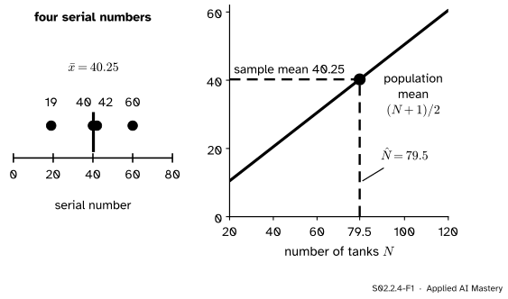
For the tanks, if the serials run from 1 to \(N\), every serial is equally likely, and their average is the middle of the range, \({(N + 1)/2}\). The four serials average 40.25.
S02.2.4-F1
The method of moments, solved by eye. The population mean \({(N + 1)/2}\) rises with \(N\); it equals the sample mean 40.25 at \({\hat{N} = 79.5}\).
Solving \({(N + 1)/2 = 40.25}\) gives \({N = 79.5}\). That is an estimator built in one line. Whether it is a good one is a separate question, and the last three lessons gave us the tools to answer it: its bias, its variance and its mean squared error.
Build it up
Step 1. Moments. The \(j\)-th population moment is \({\mu_j = \E[X^j]}\), a function of the parameters. The \(j\)-th sample moment is \({m_j = \frac{1}{n}\sum x_i^j}\). The first of each is the mean.
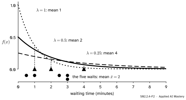
Step 2. One parameter, one equation. The exponential model of waiting times (M06.8.2) has rate \(\lambda\) and mean \({1/\lambda}\). The waiting times 1, 3, 0.5, 2.5 and 3 minutes have \({\bar{x} = 10/5 = 2}\). Setting \({1/\lambda = 2}\) gives \({\hat\lambda = 1/\bar{x} = 0.5}\) per minute.
S02.2.4-F2
Each rate \(\lambda\) gives a curve with mean \({1/\lambda}\). The one whose mean matches the sample’s, 2 minutes, is \({\lambda = 0.5}\).
Step 3. Two parameters, two equations. The normal has \({\mu_1 = \mu}\) and \({\mu_2 = \sigma^2 + \mu^2}\), since a mean square is the variance plus the squared mean. Match both:
The last step expands \({\sum (x_i - \bar{x})^2 = \sum x_i^2 - n\bar{x}^2}\). So the moment estimate of the variance divides by \(n\): the biased estimator of S02.2.1. For design A’s five times on a page (4, 5, 7, 8, 11 minutes, invented), \({m_2 = 275/5 = 55}\), so \({\hat\sigma^2 = 55 - 49 = 6}\), against \({s^2 = 7.5}\).
Step 4. A uniform. On \({[0, \theta]}\) the mean is \({\theta/2}\), so \({\hat\theta = 2\bar{x}}\). The tank serials are the same idea on the whole numbers 1 to \(N\), where the mean is \({(N + 1)/2}\) and the estimate is \({2\bar{x} - 1}\).
The formal statement
NoteDefinition: method of moments
For a model with \(q\) parameters, write the first \(q\) population moments \({\mu_1, \dots, \mu_q}\) as functions of the parameters, set each equal to the matching sample moment \({m_1, \dots, m_q}\), and solve the \(q\) equations. The solution is the method-of-moments estimator.
Why it is reasonable: by the law of large numbers each \(m_j\) settles on \(\mu_j\) as \(n\) grows, so when the equations can be solved smoothly the estimates settle on the true parameters. Moment estimators are usually consistent. They are not usually unbiased, and they need not be efficient. For the tanks we can check all three properties exactly.
The model.\(k\) tanks are captured, so \(k\) serials are drawn without replacement from \({1, \dots, N}\), every set of \(k\) equally likely.
Estimator 1: moments, \({2\bar{X} - 1}\). Each single serial is equally likely to be any of \({1, \dots, N}\), so its mean is \({(N + 1)/2}\), and by linearity \({\E[\bar{X}] = (N + 1)/2}\). Then \({\E[2\bar{X} - 1] = N}\): unbiased. Its variance uses two facts: one serial has variance \({(N^2 - 1)/12}\), and drawing without replacement multiplies the variance of a mean by the finite population correction \({(N - k)/(N - 1)}\) (S02.1.2). So
Estimator 2: the maximum \(M\). No tank numbered above \(N\) exists, so \({M \le N}\) always: it can only undershoot. Exactly how much? The maximum equals \(m\) when serial \(m\) is drawn and the other \({k - 1}\) come from the \({m - 1}\) numbers below it:
\[
\Prob(M = m) = \frac{\binom{m-1}{k-1}}{\binom{N}{k}}
\]
for \({m = k, \dots, N}\).
Multiply by \(m\) and use \({m\binom{m-1}{k-1} = k\binom{m}{k}}\), since both sides equal \({\frac{m!}{(k-1)!\,(m-k)!}}\):
The middle step is the hockey-stick identity \({\sum_{m=k}^{N}\binom{m}{k} = \binom{N+1}{k+1}}\): choose \({k + 1}\) numbers from \({1, \dots, N + 1}\) and sort the choices by their largest, \({m + 1}\); the other \(k\) come from the \(m\) numbers below. The last step cancels factorials. So \({\text{Bias}(M) = \frac{k(N + 1)}{k + 1} - N = -\frac{N - k}{k + 1}}\).
Estimator 3: the corrected maximum. Undo the bias: \({\frac{k + 1}{k}M - 1}\) has mean \({(N + 1) - 1 = N}\). Written as \({M + \frac{M - k}{k}}\) it is the maximum plus the average gap between the serials seen. Its variance, stated here and checked by exact sums in the code, is \({\frac{(N + 1)(N - k)}{k(k + 2)}}\), so the moment estimator’s variance is \({(k + 2)/3}\) times as large: twice as large for \({k = 4}\).
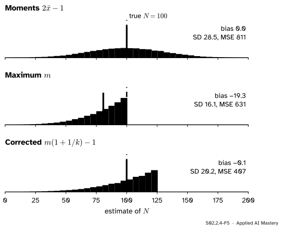
S02.2.4-F5
The three estimators over 20,000 simulated captures of four tanks from \({N = 100}\). Moments: no bias, wide. Maximum: narrow, but centred near 81. Corrected maximum: no bias and the narrowest unbiased pile.
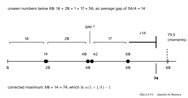
The corrected maximum read off the number line: the four serials leave 56 unseen numbers below 60, an average gap of 14, and one more gap above the largest serial gives 74.
The gap reading explains the correction. Four serials cut \({1, \dots, 60}\) into four stretches of unseen numbers, 18, 20, 1 and 17, adding to \({60 - 4 = 56}\). The unseen numbers above the maximum, up to \(N\), form a fifth stretch, and on average all five stretches have the same length. So estimate the fifth by the average of the four we can see, 14, and add it to the maximum.
Which to trust? Suppose for the check that the truth is \({N = 100}\). Exactly, with \({k = 4}\):
The corrected maximum wins, and even the biased maximum beats the unbiased moment estimate on MSE, the lesson of S02.2.3 again. The maximum carries all the information about the top end; the mean mixes it with the other serials’ positions, which say little.
Code
The three estimates, then the exact moments of each for \({N = 100}\) by summing over every possible maximum with math.comb.
import mathimport numpy as npserials = np.array([19, 40, 42, 60])k =len(serials)mom, mx =2* serials.mean() -1, serials.max()corrected = mx * (1+1/ k) -1print(f"moments {mom}, maximum {mx}, corrected maximum {corrected}")N =100p_max = {m: math.comb(m -1, k -1) / math.comb(N, k) for m inrange(k, N +1)}e_max =sum(m * p for m, p in p_max.items())var_max =sum(m * m * p for m, p in p_max.items()) - e_max **2var_corr = (1+1/ k) **2* var_maxvar_mom = (N +1) * (N - k) / (3* k)print(f"E[M] = {e_max:.1f} var(M) = {var_max:.2f} MSE(M) = {var_max + (e_max - N) **2:.1f}")print(f"var(corrected) = {var_corr:.1f} var(moments) = {var_mom:.1f}")
The formula for the variance of the moment estimator used the finite population correction. A seeded simulation checks it and the rest: 20,000 captures of four tanks from 100.
rng = np.random.default_rng(7)draws = np.argsort(rng.random((20_000, N)), axis=1)[:, :k] +1# four distinct serials per rowestimates = {"moments": 2* draws.mean(axis=1) -1,"maximum": draws.max(axis=1).astype(float),"corrected": draws.max(axis=1) * (1+1/ k) -1}for name, e in estimates.items():print(f"{name:9s} bias {e.mean() - N:6.2f} variance {e.var():6.1f} MSE {np.mean((e - N) **2):6.1f}")below = np.mean(estimates["moments"] < draws.max(axis=1))print(f"share of captures where 2 x-bar - 1 is below a serial already seen: {below:.3f}")
moments   bias  -0.00  variance  811.5  MSE  811.5
maximum   bias -19.25  variance  260.4  MSE  631.0
corrected bias  -0.06  variance  406.8  MSE  406.9
share of captures where 2 x-bar - 1 is below a serial already seen: 0.169
Last, the library. rv_continuous.fit with method="MM" matches as many moments as there are free parameters; floc=0 fixes the location at 0.
SciPy solves the moment equations numerically, so its uniform answer agrees with \({2\bar{x} = 80.5}\) to three decimals rather than exactly. It knows only the continuous uniform; the discrete serials need the \({-1}\) of the formal section.
Explore
This module’s interactive, the estimator target, is in lesson S02.2.3. It shows the same contest as the tanks on a smaller scale: an unbiased estimator against a biased one that scatters less.
Pitfalls
S02.2.4-F4
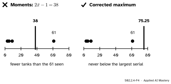
Wrong beside right. For the serials 3, 5, 9, 61 the moment estimate is 38, fewer tanks than the largest serial already seen. The corrected maximum, 75.25, can never fall below the data.
“The method of moments always gives a possible answer.”
It matches an average and ignores everything else, including what the data rule out. For the serials 3, 5, 9, 61 it says 38 tanks although tank 61 exists. In the simulation this happens in about one capture in six. Moment equations can also have no solution, or several.
“An unbiased estimator beats a biased one.”
The moment estimate is unbiased and has MSE 808 for \({N = 100}\); the plain maximum is biased by \({-19.2}\) and has MSE 627. Compare by MSE, as in S02.2.3, and then ask whether the bias can be removed, as the corrected maximum does.
“A moment estimate is only a rough guess, so it is not worth computing.”
It is quick, needs no optimiser, and is usually consistent. That makes it the standard starting point for numerical maximum likelihood: S02.3.4 starts Newton’s method for the gamma distribution from its moment estimates, \({\hat{k} = \bar{x}^2/\hat\sigma^2}\) and scale \({\hat\sigma^2/\bar{x}}\). In machine learning, the running mean and variance that batch normalisation keeps are moment estimates too: sample moments, averaged over batches.
Check yourself
Recall
1. State the method of moments in one sentence.
Show answer
Set as many population moments as there are parameters equal to the matching sample moments, and solve for the parameters.
2. What are the moment estimators of the exponential rate and of the normal variance?
Show answer
\({\hat\lambda = 1/\bar{x}}\), and \({\hat\sigma^2 = m_2 - \bar{x}^2}\), the variance with divisor \(n\).
3. What do the three tank estimators give for the serials 19, 40, 42, 60?
Show answer
Moments 79.5, maximum 60, corrected maximum 74.
4. What is the expected maximum of \(k\) serials drawn from \({1, \dots, N}\)?
Show answer
\({k(N + 1)/(k + 1)}\); for \({k = 4}\), \({N = 100}\) it is 80.8.
5. For \({N = 100}\) and \({k = 4}\), rank the three estimators by MSE.
Show answer
Corrected maximum 404, maximum 627.2, moments 808.
Exercises
1.★ A Poisson count (M06.8.3) has mean \(\lambda\). Five days give 2, 0, 3, 1 and 4 events. Find the moment estimate of \(\lambda\). Is the estimator unbiased?
Show solution
Match \({\E[X] = \lambda}\) to \({\bar{x} = 10/5 = 2}\): \({\hat\lambda = 2}\). The estimator is \(\bar{X}\), which is unbiased for the mean by S02.2.1, so it is unbiased for \(\lambda\).
2.★★ The gamma distribution with shape \(k\) and scale \(\theta\) has mean \({k\theta}\) and variance \({k\theta^2}\). Derive the moment estimators and apply them to design A’s times, with \({\bar{x} = 7}\) and \({\hat\sigma^2 = 6}\).
Show solution
Matching the mean and the variance (equivalent to matching \(m_1\) and \(m_2\)) gives \({k\theta = \bar{x}}\) and \({k\theta^2 = \hat\sigma^2}\). Dividing the second by the first gives \({\hat\theta = \hat\sigma^2/\bar{x}}\), and then \({\hat{k} = \bar{x}/\hat\theta = \bar{x}^2/\hat\sigma^2}\). For design A, \({\hat\theta = 6/7 = 0.857}\) and \({\hat{k} = 49/6 = 8.17}\).
3.★★★ Only one tank is captured, so \({k = 1}\), with serial \(m\). Show that the moment estimate and the corrected maximum agree, and that the ratio of their variances, \({(k + 2)/3}\), is then 1, as it must be.
Show solution
With one serial, \({\bar{x} = m}\), so the moment estimate is \({2m - 1}\), and the corrected maximum is \({m(1 + 1/1) - 1 = 2m - 1}\): the same rule. Its mean is \({2\,\frac{N + 1}{2} - 1 = N}\). The ratio \({(k + 2)/3}\) at \({k = 1}\) is \({3/3 = 1}\), consistent with two names for one estimator. Both variance formulas give \({(N + 1)(N - 1)/3}\) at \({k = 1}\).
Summary card
Match the population’s moments to the sample’s, solve, then judge the result by bias, variance and MSE.
S02.2.4-F1
\({(N + 1)/2 = 40.25}\) gives 79.5.
Recipe.\({\mu_j(\theta) = m_j}\) for \({j = 1, \dots, q}\); solve for \(\theta\).
Examples.\({\hat\lambda = 1/\bar{x}}\); normal: \(\bar{x}\) and divisor-\(n\) variance; uniform \({2\bar{x}}\).
Tanks.\({\E[M] = k(N + 1)/(k + 1)}\); corrected \({M(1 + 1/k) - 1}\), the best of the three.
Code.stats.expon.fit(x, floc=0, method="MM").
Sources and next steps
Sources. Each was opened and checked against this lesson on 15 November 2026.
Wikipedia, Method of moments (statistics): population moments written as functions of the parameters are set equal to the sample moments and the equations solved (section Method); under stated conditions the estimator is consistent (section Properties); the equations may have no solution or several, and the estimators are in general not asymptotically efficient (section Advantages and disadvantages).
Wikipedia, German tank problem, section Frequentist analysis, Minimum-variance unbiased estimator: the estimator \({m(1 + k^{-1}) - 1}\), described as the sample maximum plus the average gap between observations, with variance \({\frac{1}{k}\frac{(N - k)(N + 1)}{k + 2}}\).
SciPy documentation, scipy.stats.rv_continuous.fit: the method argument, “MLE” by default or “MM” for the method of moments, which matches the first raw moments of the data to those of the distribution, one for each free parameter, by minimising their relative errors; floc and fscale hold the location and scale fixed.
Next. S02.3 Maximum likelihood, the next module of this course, builds estimators a second way, by asking which parameter makes the observed data most probable.