Two unbiased estimators of the same centre can differ in how widely they scatter. Compare the mean and the median by their variances, read relative efficiency as the share of the data an estimator wastes, and see the median win when tails are heavy.
S02.2.2L2 Intermediate25 minIn review (what this means)
The maths and code on this page are checked by automated tests on every change, but an independent reader has not signed it off yet. Spot a mistake or a confusing step? Tell us.
Compare two unbiased estimators by their variances and compute their relative efficiency.
Use the large-sample variance of the median, 1 / (4 n f(m)²), to find its efficiency against the mean for normal, Laplace and t₃ populations.
Translate a relative efficiency into the number of observations one estimator needs to match the other.
Explain why the median earns its keep when a few values come from a wilder source, and check it by simulation with numpy.mean and numpy.median.
The question
A sensor reports a quantity with symmetric noise, and you take 25 readings. Both the mean and the median of the readings are unbiased for the true value, so both are right on average. Which should you report? In machine learning the same choice hides inside the loss: training with squared error predicts a mean, training with absolute error predicts a median, and the better one depends on the noise.
From the last lesson
1. Define the bias of an estimator \(\hat\theta\).
Show answer
\({\text{Bias}(\hat\theta) = \E[\hat\theta] - \theta}\), the gap between the centre of its sampling distribution and the truth.
2. What is the bias of the variance estimator with divisor \(n\)?
Show answer
\({-\sigma^2/n}\): it averages \({\frac{n-1}{n}\sigma^2}\).
Intuition
Unbiasedness only says where an estimator’s pile of answers is centred. Two estimators can share a centre and still differ in how wide the pile is, and a narrower pile means any one estimate is likely to land closer to the truth.
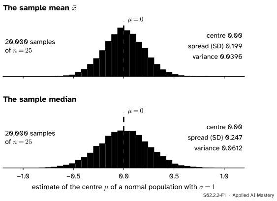
Here are both estimators applied to the same 20,000 samples of 25 readings from a normal population with centre \({\mu = 0}\) and \({\sigma = 1}\).
S02.2.2-F1
Same samples, same centre, different widths. For normal data the median’s estimates scatter more than the mean’s: a variance of 0.061 against 0.040.
The spread of an estimator’s sampling distribution is its variance, and its square root is the standard error of S02.1.2. Between two unbiased estimators, the one with the smaller variance is the better tool. Here that is the mean: the median throws away part of the information in the sample, because it listens only to the order of the values near the middle, not to how far out the others lie. Whether that is a weakness or a strength depends on the population, as the rest of this lesson shows.
Build it up
Step 1. The mean. For any population with variance \(\sigma^2\), \({\operatorname{Var}(\bar{X}) = \sigma^2/n}\) (M06.11.1). With \({\sigma = 1}\) and \({n = 25}\) that is 0.04; the simulation gives 0.0396.
Step 2. The median. No equally simple exact formula exists, but the simulation gives 0.0612, and the large-sample formula of the next section gives \({\pi/(2 \times 25) = 0.0628}\).
Step 3. Compare by a ratio. The ratio of the two variances is \({0.040/0.0628 = 2/\pi \approx 0.64}\). Read it as data: the median from 100 readings is about as precise as the mean from 64. On normal data the median wastes about a third of the sample.
Step 4. Change the population. What the median needs is many values close to the middle, since only they decide where the middle falls. What the mean fears is values far out, since each pulls it in proportion to its distance. Populations differ in both.
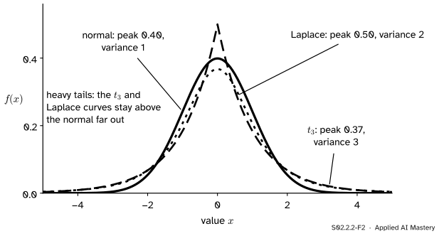
S02.2.2-F2
Three populations with the same centre. The mean’s precision depends on the variance, set by the tails; the median’s on the height of the peak \(f(0)\).
The Laplace density, \({\frac{1}{2}e^{-\abs{x}}}\), has a sharp peak and tails heavier than the normal. The \(t_3\) density (the \(t\) distribution of S02.1.4 with three degrees of freedom) has tails so heavy that its variance, 3, comes mostly from rare far values: the draws beyond \({\pm 3}\), about 6 percent of them, supply about 61 percent of it.
The formal statement
NoteDefinition: relative efficiency
For two unbiased estimators \(T_1\) and \(T_2\) of the same parameter, the efficiency of \(T_1\) relative to \(T_2\) is
A value above 1 means \(T_1\) is the more precise. \(T_1\) with \(n\) observations then matches \(T_2\) with \({\text{eff} \times n}\).
The last sentence holds whenever both variances fall like \(1/n\), as all of ours do: if \({\operatorname{Var}(T_1) = a/n}\) and \({\operatorname{Var}(T_2) = b/n}\), then \(T_2\) with \(m\) observations matches \(T_1\) with \(n\) when \({b/m = a/n}\), that is \({m = (b/a)\,n}\).
Result: the variance of the median for large \(n\). Let the population have median \(m\) and a density \(f\) that is positive and continuous at \(m\). Then for large \(n\) the sample median is approximately normal with mean \(m\) and
Why. The median is at most \({m + \delta}\) exactly when at least half the sample is at most \({m + \delta}\). The share of the sample at most \({m + \delta}\) is a sample proportion. Its mean is \({F(m + \delta) \approx \frac12 + f(m)\,\delta}\), a first-order Taylor step on the CDF \(F\) (M04.8), and its standard error is close to \({\sqrt{\frac12 \cdot \frac12 / n} = \frac{1}{2\sqrt{n}}}\) (S02.1.2). By the normal approximation for a proportion,
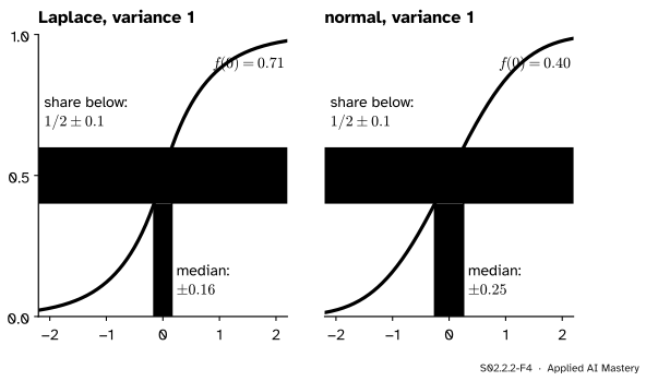
which is the CDF at \({m + \delta}\) of a normal with mean \(m\) and standard deviation \({1/(2\sqrt{n}\,f(m))}\). Squaring that standard deviation gives the result. The picture below shows the same step: a fixed wobble in the share is a small wobble in \(x\) where the CDF is steep.
S02.2.2-F4
For \({n = 25}\) the share of the sample below a point wobbles by about \({\pm 0.1}\) whatever the population. A high peak \(f(m)\) makes the CDF steep, so the median wobbles little.
The three populations. Each is symmetric, so its median is its mean and both estimators target the same number.
Normal.\({f(\mu) = \frac{1}{\sigma\sqrt{2\pi}}}\), so \({\frac{1}{4n f(\mu)^2} = \frac{2\pi\sigma^2}{4n} = \frac{\pi\sigma^2}{2n}}\). The efficiency of the median relative to the mean is \({\frac{\sigma^2/n}{\pi\sigma^2/(2n)} = \frac{2}{\pi} = 0.64}\).
Laplace with density \({\frac{1}{2b}e^{-\abs{x}/b}}\): variance \({2b^2}\) and \({f(0) = \frac{1}{2b}}\), so the median’s variance is \({b^2/n}\) against the mean’s \({2b^2/n}\). The median is twice as efficient.
\(t_3\): variance 3 and \({f(0) = 0.3676}\), so the median’s variance is \({1.85/n}\) against \({3/n}\), an efficiency of 1.62 for the median.
Go deeper: the normal is where the mean is at its best
Among all unbiased estimators of a normal mean, \(\bar{X}\) has the smallest possible variance: it reaches the Cramér-Rao lower bound of S02.10.2. So no rule can beat the mean on truly normal data, and the median’s 0.64 is the price of insurance. For the Laplace population the roles swap: the median is the maximum likelihood estimate of the centre (S02.3), and for large \(n\) its variance, about \({b^2/n}\), sits at the Cramér-Rao bound for the Laplace centre: no unbiased rule does better.
Worked example
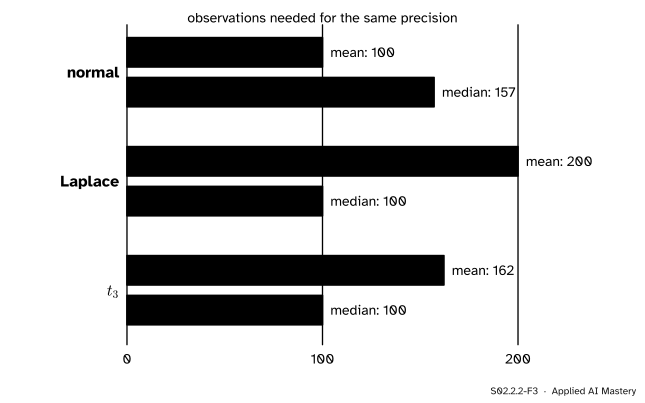
The mean of 100 readings sets a precision. How many readings does each estimator need to match the better one with 100?
S02.2.2-F3
Observations needed for equal precision. On normal data the median needs 57 percent more; on Laplace data the mean needs twice as many; on \(t_3\) data, 62 percent more.
Normal, \({\sigma = 1}\). The mean of 100 has variance \({1/100}\). The median of \(m\) has \({\pi/(2m)}\). Setting them equal gives \({m = 100\pi/2 = 157.1}\), so about 157 readings.
Laplace, \({b = 1}\). Now the median is better: with 100 readings its variance is \({1/100}\). The mean of \(m\) has \({2/m}\), and \({2/m = 1/100}\) gives \({m = 200}\).
\(t_3\). The median of 100 has \({1.85/100}\). The mean of \(m\) has \({3/m}\), so \({m = 300/1.85 = 162}\).
These are large-sample numbers. At \({n = 25}\) the simulation below finds the median’s advantage on Laplace data to be about 1.5 rather than 2: the median’s sampling distribution reaches its limit slowly when the density has a sharp peak.
Code
From scratch: draw 20,000 samples of 25 from each population, take both estimators, compare their variances.
The large-sample efficiencies, from the formula \({\operatorname{Var}(\text{median}) \approx 1/(4nf(m)^2)}\):
def eff_median(variance, peak):"""Large-n efficiency of the median relative to the mean: variance times 4 f(m)^2."""return variance *4* peak **2for name, variance, peak in [("normal", 1, stats.norm.pdf(0)), ("Laplace", 2, stats.laplace.pdf(0)), ("t3", 3, stats.t.pdf(0, 3))]: e = eff_median(variance, peak)print(f"{name:8s} f(0) = {peak:.4f} eff = {e:.3f} mean needs {100* e:.0f} to match median's 100")
normal   f(0) = 0.3989  eff = 0.637  mean needs 64 to match median's 100
Laplace  f(0) = 0.5000  eff = 2.000  mean needs 200 to match median's 100
t3       f(0) = 0.3676  eff = 1.621  mean needs 162 to match median's 100
Now outliers. Suppose 1 reading in 20 comes from a faulty source with ten times the spread: a standard normal most of the time, a normal with \({\sigma = 10}\) with chance 0.05. The mean’s variance times \(n\) becomes \({0.95 + 0.05 \times 100 = 5.95}\). The density at 0 barely falls, so the median hardly notices.
eps, k =0.05, 10rng = np.random.default_rng(3)x = rng.normal(0.0, 1.0, (reps, n))x = np.where(rng.random((reps, n)) < eps, k * x, x)var_mean, var_median = np.mean(x, axis=1).var(), np.median(x, axis=1).var()peak = stats.norm.pdf(0) * (1- eps + eps / k)print(f"n var(mean): simulated {n * var_mean:.2f}, theory {1- eps + eps * k **2:.2f}")print(f"n var(median): simulated {n * var_median:.2f}, large-n formula {1/ (4* peak **2):.2f}")print(f"the median is {var_mean / var_median:.1f} times as efficient")
n var(mean):   simulated 5.93, theory 5.95
n var(median): simulated 1.69, large-n formula 1.72
the median is 3.5 times as efficient
One faulty reading in twenty makes the median about three and a half times as efficient as the mean. This is the case S01.4.4 made for checking outliers, now in numbers.
Explore
This module’s interactive, the estimator target, is in lesson S02.2.3: it adds the third way to judge an estimator, which weighs bias and variance together.
Pitfalls
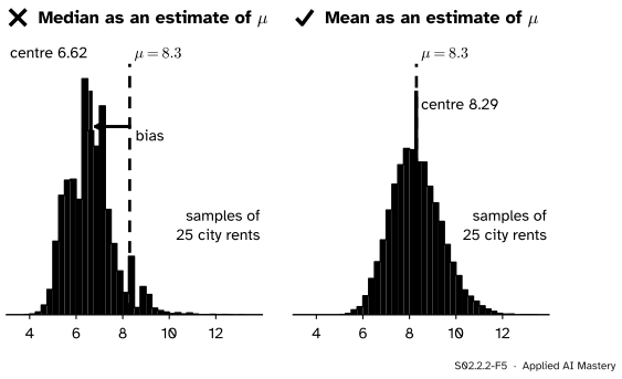
S02.2.2-F5
Wrong beside right, on the skewed city rents. The sample median centres at about 6.6, near the city’s median 6.55, not on its mean 8.3: on skewed data the two estimators aim at different targets.
“The median is a more robust estimate of the mean.”
Only when the population is symmetric, so that its median and mean coincide. The city’s rents are skewed right, with median 6.55, and medians of 25 rents centre near 6.6 against \({\mu = 8.3}\). Comparing variances is meaningful only between estimators of the same parameter; first decide which parameter the question needs.
“The median always loses, because it ignores data.”
It loses on normal data, by a factor of 0.64. It wins on heavy-tailed data and badly so when a few values come from a wilder source: 3.5 times as efficient with one faulty reading in twenty. In machine learning this is why absolute error and the Huber loss are used for targets with outliers.
“A large-sample efficiency holds at my sample size.”
The formula \({1/(4nf(m)^2)}\) is a limit. At \({n = 25}\) it is close for normal data (0.0628 against 0.0612) but promises 2 for the Laplace population where the simulation finds about 1.5. When the sample is small, simulate.
Check yourself
Recall
1. Two unbiased estimators of the same parameter: how do you decide which is better?
Show answer
Compare their variances; the one with the smaller variance scatters less around the truth.
2. Define the efficiency of \(T_1\) relative to \(T_2\).
Show answer
\({\operatorname{Var}(T_2)/\operatorname{Var}(T_1)}\). Above 1 means \(T_1\) is more precise.
3. What is the large-sample variance of the sample median?
Show answer
\({1/(4nf(m)^2)}\), where \(f(m)\) is the population density at its median.
4. What is the efficiency of the median relative to the mean for normal data, and what does it mean in observations?
Show answer
\({2/\pi \approx 0.64}\): the median needs about 157 observations to match the mean of 100.
5. For which populations does the median beat the mean?
Show answer
Symmetric populations with heavy tails or a sharp peak, such as the Laplace and \(t_3\), and data where a few values come from a much wilder source.
Exercises
1.★ A normal population has \({\sigma = 2}\). For \({n = 100}\), find the variance of the sample mean and the large-sample variance of the sample median.
Show solution
\({\operatorname{Var}(\bar{X}) = 4/100 = 0.04}\). The median’s variance is about \({\pi \times 4/(2 \times 100)}\), which is 0.0628. The ratio is again \({2/\pi}\): efficiency does not depend on \(\sigma\).
2.★★ For the uniform population on \({[0, 1]}\), find the large-sample efficiency of the median relative to the mean. Which would you use?
Show solution
The variance of one value is \({1/12}\), so \({\operatorname{Var}(\bar{X}) = 1/(12n)}\). The density is 1 everywhere on \({[0, 1]}\), so \({f(m) = 1}\) and \({\operatorname{Var}(\text{median}) \approx 1/(4n)}\). The efficiency is \({\frac{1/(12n)}{1/(4n)} = \frac{1}{3}}\). Use the mean: a flat population has no peak for the median to exploit and no tails for the mean to fear.
3.★★★ A population is standard normal with chance \({1 - \varepsilon}\) and normal with standard deviation \(k\) with chance \(\varepsilon\), both centred on 0. Show that the large-sample efficiency of the median relative to the mean is \({\frac{2}{\pi}\,(1 - \varepsilon + \varepsilon k^2)(1 - \varepsilon + \varepsilon/k)^2}\), and evaluate it for \({\varepsilon = 0.05}\), \({k = 10}\).
Show solution
The variance of the mixture is the weighted average of the two variances, since both have mean 0: \({\sigma^2 = (1 - \varepsilon) \cdot 1 + \varepsilon k^2}\). Its density at 0 is the weighted average of the two densities at 0, \({\frac{1}{\sqrt{2\pi}}}\) and \({\frac{1}{k\sqrt{2\pi}}}\):
Normal. Median efficiency \({2/\pi = 0.64}\). Laplace. 2. \(t_3\). 1.62.
Check first. Mean and median share a target only for symmetric populations.
Sources and next steps
Sources. Each was opened and checked against this lesson on 15 November 2026.
Eric W. Weisstein, Statistical Median, MathWorld: for large samples the variance of the median is \({1/(4Nf^2(\tilde{x}_0))}\) with \(f\) the density at the population median (equation 4), and the efficiency of the median, the ratio of the variance of the mean to that of the median, tends to \({2/\pi \approx 0.637}\) for a normal population.
UC Berkeley Statistics 135, Lecture 16: Efficiency: for i.i.d. \({N(\theta, 1)}\) data the sample median has variance about \({\pi/(2n)}\) for large \(n\), and its asymptotic relative efficiency against the mean is \({2/\pi \approx 0.63}\).