An estimator is a rule that turns a sample into a guess, and its guesses vary from sample to sample. Define bias as the gap between their average and the truth, prove that x-bar, p-hat and s² are unbiased, and see why s is not.
S02.2.1L2 Intermediate25 minIn review (what this means)
The maths and code on this page are checked by automated tests on every change, but an independent reader has not signed it off yet. Spot a mistake or a confusing step? Tell us.
Tell an estimator (a rule, and so a random variable) from an estimate (its value on one sample).
Define the bias of an estimator and compute it by listing every outcome of a small experiment.
Prove that the sample mean, the sample proportion and the sample variance with divisor n - 1 are unbiased, and that the divisor n falls short by sigma squared over n.
Explain why the sample standard deviation is biased low although its square is unbiased, and check it by simulation.
Choose the divisor in numpy.var, numpy.std and numpy.cov with ddof.
The question
Draw five rents at random from the city and ask for their variance. numpy.var gives one number and pandas another, because one divides the sum of squares by 5 and the other by 4. Every new sample gives new numbers again. So what can it mean for a rule like “divide by 4” to be right, when no single answer it gives is ever exactly the truth? The same question sits under every number a machine learning pipeline reports from data: a test-set accuracy, a feature’s variance used for scaling, the covariance matrix fed to PCA.
Intuition
A sample is a handful of rows drawn from something larger. A statistic turns the sample into a number, and when that number is meant as a guess at a fixed feature of the population, the rule is called an estimator and its value on one sample an estimate. The rule is fixed; the estimate changes every time the sample does.
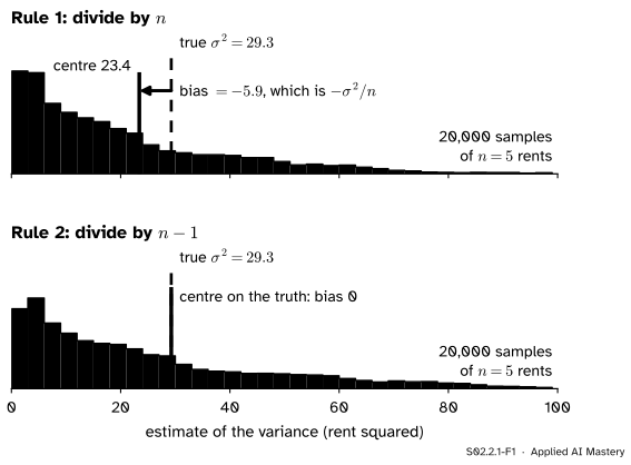
So judge the rule, not one answer: apply it to many samples and look at where the answers pile up. Below, two rules for the variance are applied to the same 20,000 samples of five rents from the city of S01 (invented, 500 flats, true variance \({\sigma^2 = 29.3}\)).
S02.2.1-F1
The same samples, two rules. Dividing the sum of squares by \(n\) gives estimates that centre at 23.4, below the truth; dividing by \({n - 1}\) gives estimates that centre on it. Neither rule is right for any one sample.
Both piles are wide: a single estimate can land anywhere from near 0 to over 100. What separates the rules is the centre of the pile. Rule 1 centres a fifth below the truth: on average it undershoots. Rule 2 centres on the truth: its misses cancel out over many samples. That gap between the centre and the truth is the bias of a rule, and a rule with no gap is unbiased. This lesson proves which rules are unbiased; the next two ask what the width of the pile costs.
Build it up
Step 1. Name the parts. The population has a fixed, unknown number we want, the parameter\(\theta\) (here the variance \(\sigma^2\), elsewhere a mean \(\mu\) or a proportion \(p\)). A sample is \({X_1, \dots, X_n}\), drawn independently from the population. An estimator \(\hat\theta\) is any function of the sample.
S02.2.1-F2
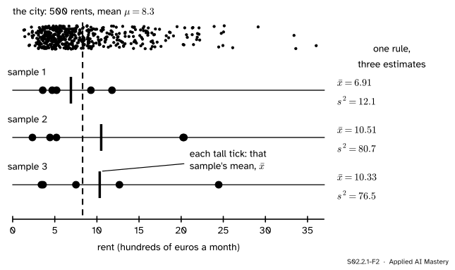
The first three samples of the simulation. One rule, the sample mean, gives three different estimates; so does the sample variance.
Step 2. An estimator is a random variable. Before the sample is drawn, \(\hat\theta\) is uncertain, so it has a distribution: its sampling distribution, drawn as the histograms above (lesson S02.1.1 of this course). After the sample is drawn we hold one number, the estimate.
Step 3. Its centre is an expectation. The centre of the pile is the expected value \(\E[\hat\theta]\), the long-run average over all possible samples.
Step 4. Bias compares the centre with the truth.\({\text{Bias}(\hat\theta) = \E[\hat\theta] - \theta}\). It is a property of the rule, never of one estimate.
The formal statement
NoteDefinitions: estimator, bias, unbiased
An estimator of a parameter \(\theta\) is a function \({\hat\theta = h(X_1, \dots, X_n)}\) of the sample. Its bias is
Result 2: the sample proportion is unbiased for \(p\). Code a success as 1 and a failure as 0. Then \(\hat{p}\) is the mean of these indicators, each with mean \({1 \cdot p + 0 \cdot (1-p) = p}\), so Result 1 gives \({\E[\hat{p}] = p}\).
Result 3: \(s^2\) is unbiased for \(\sigma^2\), for every \(n\). S01.3.3 checked this on the 25 draws of two from five flats; here is the proof. Write each distance from \(\mu\) as a distance from \(\bar{X}\) plus the gap between the two means:
Add over \({i = 1, \dots, n}\). The factor \({(\bar{X} - \mu)}\) is the same in every term, so it comes out of the middle sum, and the last term is added \(n\) times:
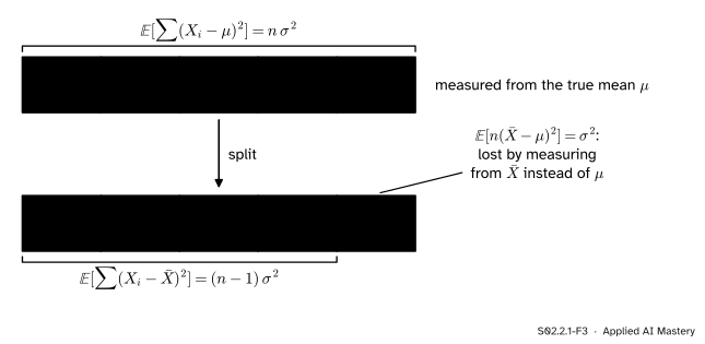
The middle sum is zero, because \({\sum X_i - n\bar{X} = 0}\). Now take expectations of what is left. Each \({\E[(X_i - \mu)^2]}\) is \(\sigma^2\), so the left side averages \({n\sigma^2}\). And \({\E[(\bar{X} - \mu)^2]}\) is the variance of \(\bar{X}\), which is \({\sigma^2 / n}\) for independent draws (M06.11.1), so the last term averages \({n \cdot \sigma^2/n = \sigma^2}\). Therefore
Dividing by \({n - 1}\) gives \({\E[s^2] = \sigma^2}\).
S02.2.1-F3
The proof as blocks, for \({n = 5}\). Measured from \(\mu\), a sample holds \(n\) blocks of \(\sigma^2\) on average. Measured from its own mean it holds one fewer, so the divisor that recovers \(\sigma^2\) is \({n - 1}\).
Result 4: the divisor \(n\) is biased. Dividing the same sum by \(n\) gives an estimator with expectation \({\frac{n-1}{n}\sigma^2}\), so its bias is
For five rents that is \({-29.3/5 = -5.9}\), the arrow in the anchor figure. The bias shrinks as \(n\) grows, which is why it hardly matters for a table of thousands of rows and matters a great deal for five. The same argument applied to products of deviations is why numpy.cov divides by \({n - 1}\) by default, as M06.10.1 promised.
Result 5: \(s\) is biased low for \(\sigma\). Unbiasedness does not survive a square root. The variance of any random variable is its mean square minus its squared mean, so
Unless every sample gives the same \(s\), this variance is positive, so \({(\E[s])^2 < \sigma^2}\) and \({\E[s] < \sigma}\). The general fact behind this is Jensen’s inequality: a curve that bends down, like the square root, pulls averages down.
Go deeper: drawing without replacement from a small population
The proof used independent draws, which is the course’s default model (S02.1.1): a city of 500 sampled five at a time is close to it. When a small population of \(N\) is used up as it is sampled, the draws are not independent, and the variance of \(\bar{X}\) is \({\frac{\sigma^2}{n}\frac{N-n}{N-1}}\) (the finite population correction of S02.1.2). Putting that into the last step gives \({\E[s^2] = \frac{N}{N-1}\sigma^2}\), with \(\sigma^2\) divided by \(N\): a slight overshoot. For the five-flat population, \({\frac{5}{4} \times 6.8 = 8.5}\), exactly the average S01.3.3 found over its ten samples without replacement.
Worked example
A coin with \({p = 0.7}\) is tossed twice. Is \(\hat{p}\) unbiased for \(p\)? Is \({\hat{p}(1 - \hat{p})}\) unbiased for \({p(1-p)}\), the variance of one toss?
There are only four outcomes, so list them all with their chances and average each estimator.
S02.2.1-F4
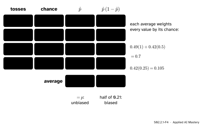
Every outcome of two tosses, weighted by its chance. \(\hat{p}\) averages exactly \({p = 0.7}\). \({\hat{p}(1-\hat{p})}\) averages 0.105, half of the true 0.21.
The chances are \({0.7^2 = 0.49}\) for two heads, \({0.7 \times 0.3 = 0.21}\) for each mixed order and \({0.3^2 = 0.09}\) for two tails. They add to 1.
\(\hat{p}\) is the share of heads: 1, 0.5, 0.5 and 0.
Weighting each value by its chance, \({\E[\hat{p}] = 0.49 + 0.21}\), which is 0.7. Unbiased, as Result 2 says.
\({\hat{p}(1-\hat{p})}\) is 0 when both tosses agree and \({0.5 \times 0.5 = 0.25}\) when they differ. Its average is \({0.42 \times 0.25 = 0.105}\), against the truth \({0.7 \times 0.3 = 0.21}\).
The second estimator is biased by \({0.105 - 0.21 = -0.105}\). This is Result 4 in disguise: \({\hat{p}(1-\hat{p})}\) is the variance of the 0s and 1s with divisor \(n\), so it averages \({\frac{n-1}{n}\,p(1-p)}\), here \({\frac{1}{2} \times 0.21}\). Multiplying by \({n/(n-1)}\) removes the bias, exactly as switching the divisor did.
Code
First the city, built as S01 builds it, and the five-rent samples of the figures.
import numpy as nprng = np.random.default_rng(0) # the city of S01, inventedparts = []for size, mean in [(250, 5.0), (150, 8.0), (100, 17.0)]: draws = rng.gamma(9.0, 1.0, size) parts.append(draws * mean / draws.mean())city = np.concatenate(parts)mu, sigma2 = city.mean(), city.var() # population: divide by Nprint(f"mu = {mu:.2f}, sigma^2 = {sigma2:.2f}, sigma = {np.sqrt(sigma2):.2f}")n =5rng = np.random.default_rng(1)samples = rng.choice(city, size=(20_000, n)) # independent draws, with replacementfor row in samples[:3]:print(f"x-bar {row.mean():.2f} s^2 {row.var(ddof=1):.1f}")
Now each rule over all 20,000 samples, from scratch, against the theory.
def sum_of_squares(x):return ((x - x.mean(axis=1, keepdims=True)) **2).sum(axis=1)ss = sum_of_squares(samples)by_n, by_n_minus_1 = ss / n, ss / (n -1)s = np.sqrt(by_n_minus_1)print(f"divide by n: average {by_n.mean():.2f}, theory {(n -1) / n * sigma2:.2f}")print(f"divide by n - 1: average {by_n_minus_1.mean():.2f}, theory {sigma2:.2f}")print(f"s: average {s.mean():.2f}, sigma {np.sqrt(sigma2):.2f}")
divide by n:     average 23.42, theory 23.41
divide by n - 1: average 29.28, theory 29.26
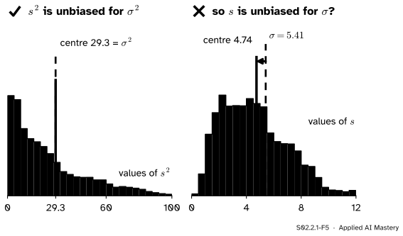
s:               average 4.74, sigma 5.41
The simulated centres sit within a tenth or two of the theory: 20,000 samples pin a centre down well but not perfectly. The coin needs no simulation, only the four outcomes.
from itertools import productp =0.7e_phat = e_prod =0.0for tosses in product([1, 0], repeat=2): chance = np.prod([p if x else1- p for x in tosses]) phat =sum(tosses) /2 e_phat += chance * phat e_prod += chance * phat * (1- phat)print(f"E[p-hat] = {e_phat:.3f} E[p-hat(1 - p-hat)] = {e_prod:.3f} p(1 - p) = {p * (1- p):.3f}")
This module’s interactive, the estimator target, lives in lesson S02.2.3. There you can shrink an unbiased estimator on purpose and watch its bias grow while its pile of estimates narrows.
Pitfalls
S02.2.1-F5
Wrong beside right. \(s^2\) centres on \(\sigma^2\), but its square root \(s\) centres at 4.74, about 12 percent below \({\sigma = 5.41}\).
“\(s^2\) is unbiased, so \(s\) is unbiased too.”
Expectation passes through sums and constant multiples, not through square roots. Result 5 shows \({\E[s] < \sigma}\) whenever \(s\) varies at all. For five city rents the shortfall is about 12 percent. It fades as \(n\) grows, and for normal data there are exact correction factors, but most software reports \(s\) uncorrected.
“An unbiased estimator gives the right answer.”
It gives the right answer on average over samples you did not draw. The first three samples above give \({s^2 = 12.1}\), 80.7 and 76.5 for a truth of 29.3. Unbiasedness says nothing about how far one estimate may land; that is the variance, the subject of the next lesson.
“np.var and np.std give the sample variance and standard deviation.”
They divide by \(n\) unless you pass ddof=1. pandas divides by \({n - 1}\) by default and numpy.cov too, so the same column can give two answers in one script. In machine learning the choice rarely matters for a large training set, but it does for small validation folds and for per-class statistics with few examples.
Check yourself
Recall
1. What is the difference between an estimator and an estimate?
Show answer
An estimator is the rule, a function of the random sample, and so a random variable. An estimate is the number the rule gives on the one sample actually drawn.
2. Define the bias of an estimator \(\hat\theta\).
Show answer
\({\text{Bias}(\hat\theta) = \E[\hat\theta] - \theta}\): the gap between the centre of its sampling distribution and the true value.
3. What is the expected value of the sum of squared deviations about \(\bar{X}\), and why does that make \({n - 1}\) the right divisor?
Show answer
\({(n-1)\sigma^2}\). Measured from \(\mu\) the sum averages \({n\sigma^2}\), and measuring from \(\bar{X}\) loses \({\E[n(\bar{X} - \mu)^2] = \sigma^2}\). Dividing \({(n-1)\sigma^2}\) by \({n - 1}\) gives \(\sigma^2\).
4. What is the bias of the variance estimator with divisor \(n\)?
Show answer
\({-\sigma^2/n}\). For samples of five city rents, about \({-5.9}\).
5. Why is \(s\) biased low for \(\sigma\)?
Show answer
Because its variance is positive whenever \(s\) varies, and
1.★ For samples of \({n = 10}\) city rents, what does the variance estimator with divisor \(n\) average, and what is its bias? Use \({\sigma^2 = 29.26}\).
Show solution
It averages \({\frac{n-1}{n}\sigma^2 = 0.9 \times 29.26 = 26.33}\), so its bias is \({26.33 - 29.26 = -2.93}\), which is \({-\sigma^2/10}\).
2.★★ For \(n\) tosses of a coin, show that \({\E[\hat{p}(1-\hat{p})] = \frac{n-1}{n}\,p(1-p)}\), and check it against the worked example.
Show solution
Write \({\hat{p}(1-\hat{p}) = \hat{p} - \hat{p}^2}\). By Result 2, \({\E[\hat{p}] = p}\). For any random variable the mean square is the variance plus the squared mean, and \({\operatorname{Var}(\hat{p}) = p(1-p)/n}\) (S02.1.2), so
so \({\bar{X}^2 - s^2/n}\) is unbiased for \(\mu^2\). It can come out negative, an early sign that an unbiased rule is not always a sensible one.
Summary card
Judge the rule by where its answers centre: bias is the centre minus the truth.
S02.2.1-F1
Divide by \({n - 1}\), and the centre is the truth.
Bias.\({\text{Bias}(\hat\theta) = \E[\hat\theta] - \theta}\); unbiased means 0 for every \(\theta\).
Unbiased.\(\bar{X}\) for \(\mu\), \(\hat{p}\) for \(p\), \(s^2\) (divisor \({n - 1}\)) for \(\sigma^2\).
Biased. Divisor \(n\): bias \({-\sigma^2/n}\). And \({\E[s] < \sigma}\).
Code.np.var(x, ddof=1); np.cov uses \({n - 1}\) by default.
Sources and next steps
Sources. Each was opened and checked against this lesson on 15 November 2026.
Hossein Pishro-Nik, Introduction to Probability, Statistics, and Random Processes, Section 8.2.1, Evaluating estimators: the definitions of bias, \({B(\hat\Theta) = \E[\hat\Theta] - \theta}\), and of an unbiased estimator, with bias zero for all possible values of \(\theta\).
The same book, Section 8.2.2, Point estimators for mean and variance: the divisor-\(n\) estimator has expectation \({\frac{n-1}{n}\sigma^2}\) and bias \({-\sigma^2/n}\), the sample variance with divisor \({n - 1}\) is unbiased, and \(S\) is a biased estimator of \(\sigma\) because \({\operatorname{Var}(S) > 0}\) gives \({\E[S] < \sigma}\).
NumPy documentation, numpy.var: the divisor is \(N\) minus ddof, ddof=0 by default, and ddof=1 gives the unbiased estimate (Bessel’s correction). numpy.cov: normalisation by \({N - 1}\) by default, by \(N\) with bias=True, and ddof overrides both.