Two coins can give the same estimate with very different precision, and the difference is written in how sharply the log-likelihood bends. Meet the score, prove that it averages zero at the truth, and measure information as its variance or as the expected curvature.
S02.10.1L2 Intermediate25 minIn review (what this means)
The maths and code on this page are checked by automated tests on every change, but an independent reader has not signed it off yet. Spot a mistake or a confusing step? Tell us.
Define the score as the slope of the log-likelihood and prove that its expectation is zero at the true parameter.
Define Fisher information as the variance of the score and derive the second form, minus the expected second derivative.
Compute the information of a coin toss, 1 / (p(1 - p)), and of an exponential waiting time, 1 / lambda squared, both ways.
Explain why information adds over independent observations and why a sharper log-likelihood means a more precise estimate.
The question
One coin lands heads 7 times in 10 tosses; another lands heads 28 times in 40. Both give the same maximum likelihood estimate, \({\hat{p} = 0.7}\), yet nobody would trust the two equally. Where in the likelihood is the difference written, and can it be measured by one number before a single toss is made? The same number later gives every fitted model its standard errors and steers the natural gradient of reinforcement learning.
Intuition
Module S02.3 found an estimate at the top of the log-likelihood. This module asks how sure that top is. Draw the two coins’ curves, each measured from its own peak, and the answer is in their shape.
S02.10.1-F1
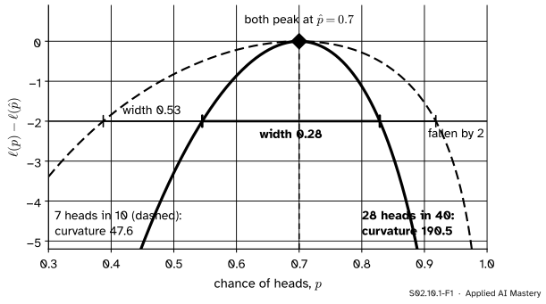
The same estimate from 10 tosses (dashed) and from 40 (solid). Four times the tosses give four times the curvature at the peak, and the band of values within 2 of the top is about half as wide.
The wide curve barely changes as \(p\) moves away from 0.7: the data from 10 tosses hardly prefer 0.7 to 0.55 or 0.85. The narrow curve drops fast, so the 40 tosses rule those values out. How fast a curve bends at its top is its curvature, minus the second derivative. Its expected value is called the Fisher information, and it is the number we were looking for: a sharp peak means a precise estimate.
Build it up
Step 1. The score. The slope of the log-likelihood has a name of its own, the score,
\[
U(\theta) = \ell'(\theta).
\]
For \(k\) heads in \(n\) tosses, \({\ell(p) = k \ln p + (n - k)\ln(1 - p)}\), so
The second form puts both fractions over \({p(1 - p)}\). The MLE is where the score is zero: \({k = np}\), so \({\hat{p} = k/n}\).
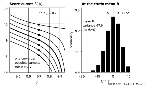
Step 2. Before the data, the score is random. Fix \({p = 0.7}\) and imagine the 10 tosses not yet made. The count \(k\) is random, so \({U(0.7) = (k - 7)/0.21}\) is a random variable too. Each possible sample draws its own score curve, and each curve cuts the line \({p = 0.7}\) at its own height.
S02.10.1-F2
Left: the score curve of each possible sample of 10 tosses, and where it crosses the true \({p = 0.7}\). Right: the exact distribution of those crossing heights. They balance at 0, and their spread, variance 47.6, is the information in 10 tosses.
Step 3. At the true value it averages zero. If the coin really has \({p = 0.7}\), the count has mean \({\E[k] = np}\), so the numerator \({k - np}\) averages zero and so does the score. The curves in the picture cross the truth sometimes above, sometimes below, and on average exactly at zero.
Step 4. Its spread is the information. The variance of the count is \({np(1 - p)}\), and dividing by the constant \({p(1 - p)}\) divides the variance by its square:
Its expected value, with \({\E[k] = np}\), is \({n/p + n/(1 - p) = n/(p(1 - p))}\), which is again 47.6. Two different questions, “how much does the score wobble?” and “how sharply does the curve bend on average?”, have one answer. That is not luck, as the formal statement shows.
The formal statement
NoteDefinition: score and Fisher information
Let one observation \(X\) have density (or probability) \({f(x \mid \theta)}\), and write \({\ell_1(\theta) = \ln f(X \mid \theta)}\) for its log-likelihood. The score is \({U_1(\theta) = \ell_1'(\theta)}\). The Fisher information in one observation is
where the subscript says that \(X\) is drawn with parameter \(\theta\). For \(n\) independent observations the score is \({U(\theta) = \ell'(\theta)}\) and the information is \({I_n(\theta)}\).
The results below need regularity conditions: the set of possible \(x\) must not depend on \(\theta\), \(\theta\) must lie inside its range rather than on an edge, and we must be allowed to differentiate under the integral sign. Lesson S02.10.2 shows what goes wrong without the first.
Result 1: the score has mean zero. Every density integrates to 1, whatever \(\theta\) is:
\[
\int f(x \mid \theta)\, dx = 1 .
\]
Differentiate both sides with respect to \(\theta\), taking the derivative inside the integral:
By the chain rule, the derivative of \({\ln f}\) is the derivative of \(f\) divided by \(f\), so \({\partial f / \partial\theta = f \cdot \partial \ln f / \partial\theta}\). Substituting,
and the left side is the definition of \({\E_\theta[U_1(\theta)]}\). So the score averages zero at the parameter the data come from. Because its mean is zero, its variance is simply \({I(\theta) = \E_\theta[U_1(\theta)^2]}\).
Result 2: information is the expected curvature. Differentiate the last integral once more. The product rule gives two terms:
In the second term replace \({\partial f / \partial\theta}\) by \({f \cdot \partial \ln f/\partial\theta}\) again. It becomes \({\int (\partial \ln f/\partial\theta)^2 f\,dx = \E_\theta[U_1^2]}\), and the first term is \({\E_\theta[\ell_1'']}\). So \({0 = \E_\theta[\ell_1''] + \E_\theta[U_1^2]}\), that is,
Result 3: information adds. For independent observations the log-likelihood is a sum, so the score is a sum of \(n\) independent scores, each with mean zero and variance \({I(\theta)}\). Variances of independent terms add (M06.7):
\[
I_n(\theta) = n\, I(\theta).
\]
Ten tosses carry ten times the information of one. In a picture, the curvature of the whole log-likelihood grows in proportion to \(n\).
S02.10.1-F5
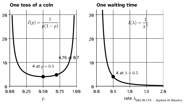
Information depends on where the parameter is. A coin toss is least informative at \({p = 0.5}\) and most informative near 0 or 1; a waiting time says more about a small rate than a large one.
Several parameters. With a vector of parameters the information becomes a matrix, minus the expected Hessian (M05.5) of \({\ell_1}\). For one normal observation with parameters \(\mu\) and \({v = \sigma^2}\),
Using \({\E[X - \mu] = 0}\) and \({\E[(X - \mu)^2] = v}\), their expectations are \({-1/v}\), 0, and \({1/(2v^2)} - {v/v^3} = {-1/(2v^2)}\).
Minus these expectations are the entries of \(\mat{I}(\mu, v)\).
Worked example
Compute the information in one toss at \({p = 0.7}\) both ways, then in ten tosses.
S02.10.1-F3
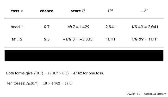
One toss has two outcomes. Weighting each by its chance gives a score that averages 0 and an information of 4.762, whether it is computed from \({U^2}\) or from \({-\ell''}\).
Log-likelihood of one toss.\({\ell_1(p) = x \ln p + (1 - x)\ln(1 - p)}\), with \({x = 1}\) for a head and \({x = 0}\) for a tail.
Score.\({U_1 = x/p - (1 - x)/(1 - p)}\): \({1/0.7 = 1.429}\) after a head, \({-1/0.3 = -3.333}\) after a tail.
Mean.\({0.7 \times 1.429} + {0.3 \times (-3.333)} = 1 - 1 = 0\), as Result 1 promised.
Variance.\({0.7 \times 1.429^2} + {0.3 \times 3.333^2}\), which is \(1.429 + 3.333 = 4.762\).
Curvature.\(-\ell_1'' = {x/p^2} + {(1 - x)/(1 - p)^2}\): 2.041 after a head and 11.111 after a tail, with average \({0.7 \times 2.041} + {0.3 \times 11.111} = 4.762\) again.
In general.\(I(p) = 1/p + {1/(1 - p)}\), which is \({1/(p(1 - p))}\), and \({1/0.21 = 4.762}\).
Ten tosses.\({I_{10}(0.7) = 10 \times 4.762 = 47.6}\), the variance in the build-up figure.
The waiting times. One exponential waiting time has \({\ell_1(\lambda) = \ln \lambda - \lambda x}\), so \({U_1 = 1/\lambda - x}\). Its mean is \({1/\lambda - \E[X] = 0}\), since an exponential waiting time has mean \({1/\lambda}\), and its variance is \({\operatorname{Var}(X) = 1/\lambda^2}\). The curvature is \({-\ell_1'' = 1/\lambda^2}\) for every \(x\), so the second form needs no averaging at all. At \({\lambda = 0.5}\) one waiting time carries information 4, and the five waiting times of the course (1, 3, 0.5, 2.5 and 3 minutes, invented) carry \({I_5 = 20}\).
Code
From scratch: list every outcome of 10 tosses, weight it by its binomial probability, and average the score, its square and the curvature at \({p = 0.7}\).
import mathimport numpy as npn, p =10, 0.7ks =range(n +1)prob = [math.comb(n, k) * p**k * (1- p)**(n - k) for k in ks]score = [k / p - (n - k) / (1- p) for k in ks]curv = [k / p**2+ (n - k) / (1- p)**2for k in ks]mean_U =sum(w * u for w, u inzip(prob, score))E_U2 =sum(w * u * u for w, u inzip(prob, score))E_curv =sum(w * c for w, c inzip(prob, curv))print("E[U] =", round(mean_U, 12), " E[U^2] =", round(E_U2, 3), " E[-ell''] =", round(E_curv, 3))print("formula n / (p(1 - p)) =", round(n / (p * (1- p)), 3), " one toss:", round(1/ (p * (1- p)), 3))
E[U] = -0.0   E[U^2] = 47.619   E[-ell''] = 47.619
formula n / (p(1 - p)) = 47.619   one toss: 4.762
Now the waiting times, by simulation: 20,000 samples of five waiting times with rate 0.5 (seed 10), and the score of each sample at the true rate.
rng = np.random.default_rng(10)lam, m =0.5, 5x = rng.exponential(1/ lam, size=(20_000, m))U = m / lam - x.sum(axis=1) # score of the sample: n / lambda - sum of xprint("mean of the scores:", round(float(U.mean()), 2), " variance:", round(float(U.var()), 2)," theory n / lambda^2 =", m / lam**2)
mean of the scores: -0.0 variance: 19.96 theory n / lambda^2 = 20.0
The simulated mean is within a few hundredths of 0 and the variance within a few tenths of 20; a different seed moves both slightly. SciPy’s frozen distributions have an expect method that does the weighted average for us.
from scipy import statsI10 = stats.binom(10, 0.7).expect(lambda k: ((k -7) /0.21) **2)I1_exp = stats.expon(scale=2).expect(lambda t: (1/0.5- t) **2)print("coin, ten tosses:", round(I10, 3), " one waiting time at rate 0.5:", round(I1_exp, 3))
coin, ten tosses: 47.619 one waiting time at rate 0.5: 4.0
Explore
This module’s interactive, curvature and intervals, lives in lesson S02.10.4. Before you go, predict: if the coin shows 70 heads in 100 tosses, by what factor does the curvature at the peak grow compared with 7 in 10?
Pitfalls
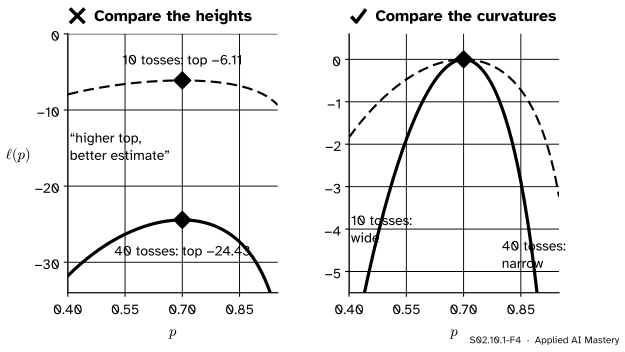
S02.10.1-F4
Wrong beside right. The height of a log-likelihood’s top falls as data are added, because every observation adds a negative log-probability. Precision is read from the bend, not the height.
“The higher the peak of the log-likelihood, the better the estimate.”
The height depends on how many observations there are and on constants that do not involve the parameter. With 40 tosses the top is at \(-24.43\), far below the \(-6.11\) of 10 tosses, yet the estimate is twice as precise. Compare curves only after shifting each to its own peak, and read precision from the curvature.
“The score is zero at the true parameter.”
The score is zero at the estimate: that is how the MLE is found. At the true value it is zero only on average over repeated samples. For any one sample it is off, by about one standard deviation, \({\sqrt{47.6} = 6.9}\) for 10 tosses, and that wobble is exactly what the information measures.
“Fisher information is computed from my data set.”
\(I(\theta)\) is an expectation over data that could be drawn with parameter \(\theta\), so it is a property of the model at a parameter value, not of one sample. The data’s own version is the observed information\({J(\hat{\theta}) = -\ell''(\hat{\theta})}\), the curvature of the curve you actually have. For the coin and the waiting times the two agree at the MLE; for many models they do not, and lesson S02.10.3 says which to use.
Check yourself
Recall
1. What is the score, and where is it zero for a given sample?
Show answer
The slope of the log-likelihood, \({U(\theta) = \ell'(\theta)}\). It is zero at the maximum likelihood estimate.
2. What is the mean of the score at the true parameter, and why?
Show answer
Zero. Differentiating \({\int f(x \mid \theta)\,dx = 1}\) with respect to \(\theta\) gives \({\int (\partial \ln f/\partial\theta) f\, dx = 0}\), which is \({\E_\theta[U_1] = 0}\).
3. Give the two forms of the Fisher information of one observation.
Show answer
\({I(\theta) = \operatorname{Var}_\theta(U_1) = \E_\theta[U_1^2]}\) and \({I(\theta) = -\E_\theta[\ell_1'']}\).
4. What is the information in one toss of a coin with chance \(p\), and in 10 tosses at \({p = 0.7}\)?
Show answer
\({I(p) = 1/(p(1 - p))}\), which is 4.762 at 0.7; ten tosses carry \({10 \times 4.762 = 47.6}\).
5. What is the information in one exponential waiting time with rate \(\lambda\)?
Show answer
\({I(\lambda) = 1/\lambda^2}\): 4 at \({\lambda = 0.5}\), and 20 for five waiting times.
Exercises
1.★ A Poisson count has \(P(X = x) = {\lambda^x e^{-\lambda}/x!}\). Find the score of one count and its information, by both forms.
Show solution
\(\ell_1 = {x \ln\lambda} - \lambda - {\ln x!}\), so \({U_1 = x/\lambda - 1}\). Its mean is \({\E[X]/\lambda - 1 = 0}\), and its variance is \({\operatorname{Var}(X)/\lambda^2}\)\(= {\lambda/\lambda^2} = {1/\lambda}\). The curvature is \({-\ell_1'' = x/\lambda^2}\), with expectation \({\lambda/\lambda^2 = 1/\lambda}\). Both forms give \({I(\lambda) = 1/\lambda}\).
2.★★ A coin lands heads 70 times in 100 tosses. Find the curvature of the log-likelihood at its peak and compare it with 7 heads in 10. By what factor is the band of \({p}\) within 2 of the top narrower, if the curve is treated as a parabola?
Show solution
At \({\hat{p} = 0.7}\), \(-\ell''(\hat p) = {70/0.49} + {30/0.09}\), which is \(142.86 + 333.33 = 476.2\), ten times the 47.6 of 10 tosses. A parabola \({-\tfrac12 J (p - \hat p)^2}\) falls by 2 at \({\abs{p - \hat p} = \sqrt{4/J}}\), so the band shrinks by \({\sqrt{10} \approx 3.16}\): from about \({\pm 0.29}\) to about \({\pm 0.092}\).
3.★★★ Describe the waiting times by their mean \({\mu = 1/\lambda}\) instead of the rate, so that \({f(x \mid \mu) = e^{-x/\mu}/\mu}\). Find \({I(\mu)}\) directly, and show that it equals \({I(\lambda)\,(d\lambda/d\mu)^2}\).
Show solution
\({\ell_1 = -\ln\mu - x/\mu}\), so \(U_1 = {-1/\mu} + {x/\mu^2} = {(x - \mu)/\mu^2}\). Its variance is \({\operatorname{Var}(X)/\mu^4} = {\mu^2/\mu^4} = {1/\mu^2}\), so \({I(\mu) = 1/\mu^2}\).
With \({\lambda = 1/\mu}\), \({d\lambda/d\mu = -1/\mu^2}\), and
The two agree. In general the score in \(\mu\) is the score in \(\lambda\) times \({d\lambda/d\mu}\) (the chain rule), so its variance picks up the square of that factor.
Summary card
Information is the expected curvature of the log-likelihood: a sharper peak, a more precise estimate.
S02.10.1-F1
Same estimate, different information.
Score.\({U(\theta) = \ell'(\theta)}\), with \({\E_\theta[U] = 0}\) at the truth.
Coin and waiting time.\({I(p) = 1/(p(1-p))}\); \({I(\lambda) = 1/\lambda^2}\).
Sources and next steps
Sources. Each was opened and checked against this lesson on 15 November 2026.
Stanford STATS 200, Autumn 2016, Lecture 14: Consistency and asymptotic normality of the MLE. Theorem 14.1 defines the score and the Fisher information by its two equivalent expressions; Lemma 14.1 proves that the score has mean zero and variance minus the expected second derivative, by differentiating the integral of the density, the proof given here.
Stanford STATS 200, Autumn 2016, Lecture 15: Fisher information and the Cramer-Rao bound. Section 15.1 gives the information matrix of several parameters (equation 15.1, as covariances of the score or minus expected second derivatives); Section 15.2 reads the information as the expected curvature of the log-likelihood, a sharp curve meaning much information.
Philippe Rigollet, Maximum likelihood estimation slides, MIT OpenCourseWare 18.650, Fall 2016. Slide 22 defines the Fisher information as the covariance of the gradient of the one-observation log-likelihood and as minus its expected Hessian, and for one parameter as \({\operatorname{var}[\ell'(\theta)] = -\E[\ell''(\theta)]}\).