\( \newcommand{\vect}[1]{\boldsymbol{\mathbf{#1}}} \newcommand{\mat}[1]{\boldsymbol{\mathbf{#1}}} \newcommand{\R}{\mathbb{R}} \newcommand{\E}{\mathbb{E}} \newcommand{\Prob}{\mathbb{P}} \newcommand{\T}{^{\top}} \newcommand{\norm}[1]{\lVert #1 \rVert} \newcommand{\abs}[1]{\lvert #1 \rvert} \newcommand{\ihat}{\mkern1mu\hat{\boldsymbol{\imath}}\mkern2mu} \newcommand{\jhat}{\mkern1mu\hat{\boldsymbol{\jmath}}\mkern2mu} \newcommand{\pd}[2]{\frac{\partial #1}{\partial #2}} \newcommand{\argmax}{\operatorname*{arg\,max}} \newcommand{\argmin}{\operatorname*{arg\,min}} \newcommand{\cdata}[1]{\class{c-data}{#1}} \newcommand{\cmodel}[1]{\class{c-model}{#1}} \newcommand{\ctruth}[1]{\class{c-truth}{#1}} \newcommand{\cgrad}[1]{\class{c-grad}{#1}} \newcommand{\closs}[1]{\class{c-loss}{#1}} \newcommand{\cparam}[1]{\class{c-param}{#1}} \newcommand{\csecond}[1]{\class{c-second}{#1}} \renewcommand{\,}{\mkern3mu} \)

The shape of a sampling distribution

Watch the central limit theorem work on skewed rents: the skewness of a mean falls like 1/√n, derived from the third moment of a sum. Judge the normal approximation by its tails, treat a proportion as a mean, and see the median settle into a bell while the maximum never does.

S02.1.3L2 Intermediate25 min

In review (what this means)

The maths and code on this page are checked by automated tests on every change, but an independent reader has not signed it off yet. Spot a mistake or a confusing step? Tell us.

Before this lesson: S02.1.2 The standard error

What you will be able to do

• Derive that the skewness of a mean of n i.i.d. draws is the skewness of one draw divided by √n.
• Judge a normal approximation to a sampling distribution by comparing its tail areas with simulated ones.
• Treat a sample proportion as a mean of indicators and say when its sampling distribution is close to normal.
• Simulate the sampling distributions of the median and the maximum, and explain why the maximum’s is not normal.

The question

City rents are badly skewed: most flats are cheap and a few in Centre are very dear. Is the mean of 5 rents close enough to normal to use the bell curve on it? The mean of 25? And what about other statistics, such as the median rent of a sample, or the highest rent in it? The answers decide when “plus or minus 1.96 standard errors” can be trusted, for a mean rent or for a model’s test accuracy.

From the last lesson

1. What is \(\operatorname{SE}(\bar{x})\) for i.i.d. draws, and how does it change when \(n\) is multiplied by four?

Show answer

\(\sigma / \sqrt{n}\); it halves.

2. What is the standard error of a sample proportion?

Show answer

\(\sqrt{p(1 - p)/n}\), because a proportion is a mean of 0s and 1s with variance \(p(1 - p)\).

Intuition

The last lesson measured how wide the sampling distribution of \(\bar{x}\) is. Its shape changes too. Standardise the mean, subtract \(\mu\) and divide by the standard error, so that every \(n\) is drawn on the same scale, and watch the lean of the city’s rents fade.

S02.1.3-F1

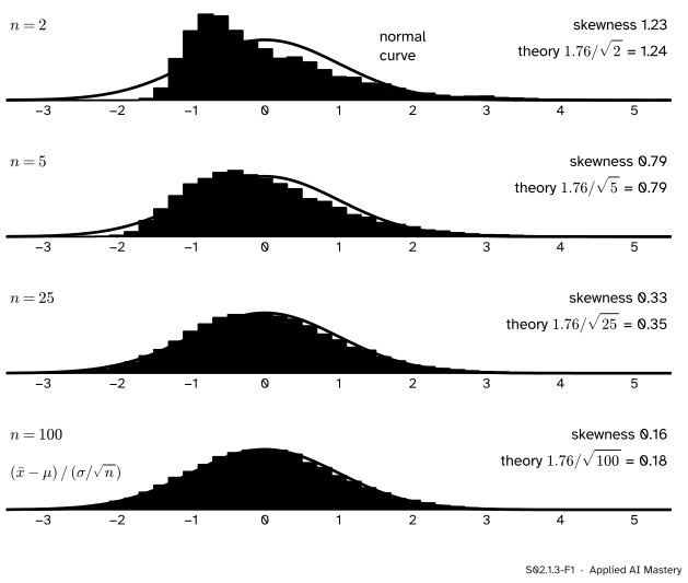
The mean of \(\cparam{n}\) city rents, standardised, for \(n = 2, 5, 25\) and 100, with the normal curve over each. The lopsidedness, measured by the skewness, falls like \(1/\sqrt{n}\).

This is the central limit theorem of M06.11.3 at work on data we care about. The theorem says the bell arrives eventually. The picture says how fast: at \(n = 2\) the mean is still lopsided, by \(n = 25\) the bell is close, and by \(n = 100\) the difference is hard to see. The speed is set by how skewed one rent is.

Build it up

Step 1. Measure the lean. The skewness of a random variable \(X\) with mean \(\mu\) and standard deviation \(\sigma\) is

\[ \gamma = \frac{\E[(X - \mu)^3]}{\sigma^3} . \]

Cubing keeps the sign, so values far above the mean push \(\gamma\) up and values far below push it down. A symmetric distribution has \(\gamma = 0\). The city’s rents have \(\gamma = 1.76\): a long tail to the right (M06.7.4 met this measure).

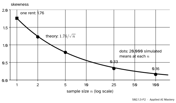
Step 2. Predict the lean of a mean. The formal section below derives that the mean of \(n\) i.i.d. draws has skewness \(\gamma / \sqrt{n}\). For the city that is 1.24 at \(n = 2\), 0.79 at \(n = 5\), 0.35 at \(n = 25\) and 0.18 at \(n = 100\).

Step 3. Check it by simulation. Twenty thousand means at each \(n\), drawn with replacement, give skewness 1.23, 0.79, 0.33 and 0.16. The law holds, within the noise of estimating a third moment.

S02.1.3-F2

The skewness of the mean of \(n\) city rents: the derived law \(1.76/\sqrt{n}\) (black) and simulation (blue dots). Halving the skewness takes four times the data, the same square-root law as the standard error.

Step 4. Judge the approximation where it is used. A bell that looks right in the middle can be wrong in the tails, and the tails are what intervals and tests use. So judge it there: compare the share of simulated means beyond \(\mu \pm {1.96\,\operatorname{SE}}\) with the 0.025 on each side that the normal curve promises. The worked example does this at \(n = 25\).

The formal statement

NoteResult: the skewness of a mean

If \(X_1, \dots, X_n\) are i.i.d. with mean \(\mu\), standard deviation \(\sigma\) and skewness \(\gamma\), then the skewness of \(\bar{X}\), and of the sum \(S = X_1 + \cdots + X_n\), is

\[ \gamma_{\bar{X}} = \frac{\gamma}{\sqrt{n}} . \]

Derivation. Write \(D_i = X_i - \mu\). The \(D_i\) are independent with \(\E[D_i] = 0\), \(\E[D_i^2] = \sigma^2\) and \(\E[D_i^3] = \gamma\sigma^3\). The sum’s distance from its mean is \(S - n\mu = D_1 + \cdots + D_n\). Expanding a cube of a sum gives three kinds of term:

\[ \begin{aligned} \Big(\sum_i D_i\Big)^3 &= \sum_i D_i^3 + 3 \sum_{i \ne j} D_i^2 D_j \\ &\quad + 6 \sum_{i < j < k} D_i D_j D_k . \end{aligned} \]

(With two terms this is \({(a + b)^3} = {a^3 + b^3 + 3a^2 b + 3ab^2}\).) Take expectations. For \(i \ne j\), independence lets the expectation split: \({\E[D_i^2 D_j]} = {\E[D_i^2]\,\E[D_j]} = {\sigma^2 \cdot 0} = 0\). In the same way every \(\E[D_i D_j D_k]\) is 0. Only the \(n\) cubes survive:

\[ \E[(S - n\mu)^3] = n\,\gamma\sigma^3 . \]

The variance of the sum is \(n\sigma^2\) (lesson S02.1.2), so its standard deviation is \(\sigma\sqrt{n}\) and

\[ \begin{aligned} \gamma_S &= \frac{n\,\gamma\sigma^3}{(\sigma\sqrt{n})^3} = \frac{n\,\gamma\sigma^3}{n^{3/2}\sigma^3} \\ &= \frac{\gamma}{\sqrt{n}} . \end{aligned} \]

Dividing \(S\) by \(n\) to get \(\bar{X}\) divides the cube on top by \(n^3\) and the standard deviation cubed below by \(n^3\), so the skewness does not change.

The proportion is a mean too. A sample proportion \(\hat{p}\) is the mean of indicators that are 1 with chance \(p\), so all of the above applies to it. One indicator has mean \(p\), and its cubed distance from \(p\) is \((1 - p)^3\) with chance \(p\) and \((-p)^3\) with chance \(1 - p\):

\[ \begin{aligned} &\E[(X - p)^3] \\ &\quad= p(1 - p)^3 - (1 - p)p^3 \\ &\quad= p(1 - p)\big[(1 - p)^2 - p^2\big] \\ &\quad= p(1 - p)(1 - 2p) . \end{aligned} \]

The last line uses \(a^2 - b^2 = (a - b)(a + b)\) with \(a + b = 1\). Dividing by \(\sigma^3 = (p(1 - p))^{3/2}\) gives the skewness of one indicator:

\[ \gamma = \frac{1 - 2p}{\sqrt{p(1 - p)}} . \]

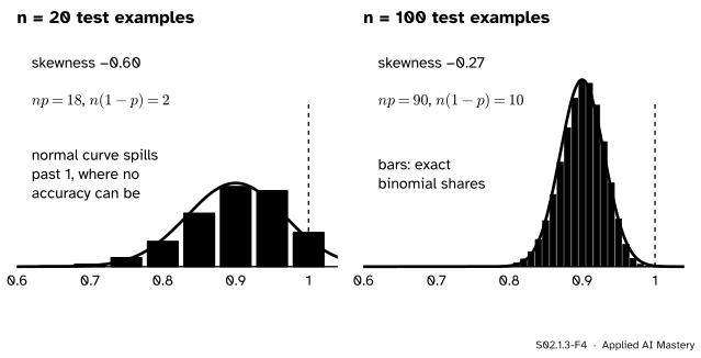
A test example answered correctly with \(p = 0.9\) has \(\gamma = -0.8 / 0.3 = -2.67\): strongly skewed to the left, because accuracies pile up against 1. So \(\hat{p}\) needs a large \(n\) before it looks normal.

S02.1.3-F4

Test-set accuracy as a mean of 0s and 1s, true accuracy \(p = 0.9\). With 20 examples the bars lean left and the normal curve puts weight above 1. With 100 the bell fits. OpenIntro’s rule of thumb asks for \(np \ge 10\) and \(n(1 - p) \ge 10\), which \(n = 100\) just meets.

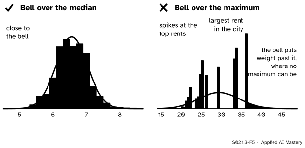
Statistics with no friendly formula. The median and the maximum are not means, so neither the \(\sigma/\sqrt{n}\) law nor the skewness law applies to them. Simulation still does. At \(n = 25\) the median of the city’s rents is more lopsided than the mean (skewness 0.76 against 0.33), but by \(n = 100\) it has settled close to a bell (0.14). The maximum never does: the pitfalls below show why.

Worked example

Is the bell good enough for the mean of 25 rents?

Predict the skewness. \({\gamma / \sqrt{25}} = {1.76 / 5} = 0.35\). Not zero, so expect some lean.

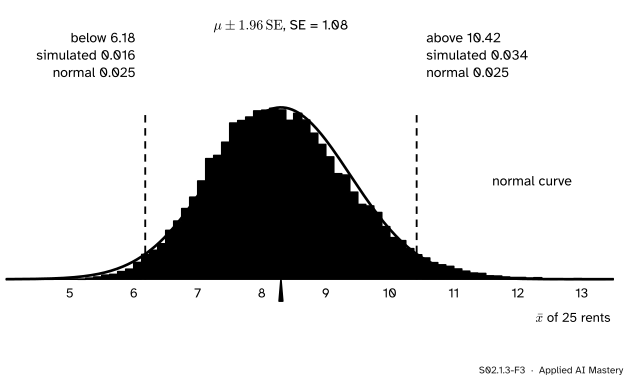
Find the cut-offs. \(\operatorname{SE} = {5.41 / 5} = 1.082\), so the normal curve puts 0.025 below \(8.3 - 1.96 \times 1.082 = 6.18\) and 0.025 above \({8.3 + 1.96 \times 1.082} = 10.42\).

S02.1.3-F3

The mean of 25 rents against its normal approximation. The bell gets the middle right but not the tails: the lower tail holds 0.016 and the upper 0.034, against 0.025 each.

Count the simulated tails. Of 20,000 simulated means, a share 0.016 fall below 6.18 and 0.034 fall above 10.42.

Read the result. Both tails together hold \(0.016 + 0.034 = 0.050\), so a two-sided “95 percent” statement is right overall. But each side is off by about a third: the mean overshoots more often than it undershoots, because the dear flats of Centre sometimes land in the sample. At \(n = 100\) the tails are 0.021 and 0.030: closer, not yet equal, as the skewness of 0.18 predicts.

Code

From scratch: the skewness of the rents with the formula of Step 1 (divisor \(N\), which is also what scipy.stats.skew computes by default, with bias=True), then the simulation.

import math
import numpy as np
from scipy import stats

rng = np.random.default_rng(0)
rents = []
for size, district_mean in ((250, 5), (150, 8), (100, 17)):
    draws = rng.gamma(9.0, 1.0, size)
    rents.append(draws * district_mean / draws.mean())
rents = np.concatenate(rents)
mu, sigma = rents.mean(), rents.std()

def skewness(x):
    d = x - x.mean()
    return np.mean(d ** 3) / np.mean(d ** 2) ** 1.5

gamma = skewness(rents)
print(f"skewness of one rent: {gamma:.2f} (scipy: {stats.skew(rents):.2f})")

rng = np.random.default_rng(5)
sims = {n: rng.choice(rents, size=(20_000, n)).mean(axis=1) for n in (2, 5, 25, 100)}
for n, means in sims.items():
    z = (means - mu) / (sigma / math.sqrt(n))
    print(f"n = {n:3d}: skewness {skewness(means):.2f} (theory {gamma / math.sqrt(n):.2f}), "
          f"below -1.96: {np.mean(z < -1.96):.3f}, above 1.96: {np.mean(z > 1.96):.3f}")

skewness of one rent: 1.76 (scipy: 1.76)
n =   2: skewness 1.23 (theory 1.24), below -1.96: 0.000, above 1.96: 0.048
n =   5: skewness 0.79 (theory 0.79), below -1.96: 0.001, above 1.96: 0.043
n =  25: skewness 0.33 (theory 0.35), below -1.96: 0.016, above 1.96: 0.034
n = 100: skewness 0.16 (theory 0.18), below -1.96: 0.021, above 1.96: 0.030

A proportion, exactly, with math.comb: the accuracy on \(n\) test examples when the true accuracy is 0.9.

p = 0.9
gamma_one = (1 - 2 * p) / math.sqrt(p * (1 - p))
for n in (20, 100):
    pmf = [math.comb(n, k) * p ** k * (1 - p) ** (n - k) for k in range(n + 1)]
    print(f"n = {n}: skewness {gamma_one / math.sqrt(n):.2f}, P(p-hat = 1) = {pmf[-1]:.3f}")

n = 20: skewness -0.60, P(p-hat = 1) = 0.122
n = 100: skewness -0.27, P(p-hat = 1) = 0.000

The median and the maximum, simulated, with the share of maxima that hit the largest rent in the city and the weight a normal curve with the same mean and standard deviation puts above it.

rng = np.random.default_rng(6)
order = {}
for n in (25, 100):
    draws = rng.choice(rents, size=(20_000, n))
    med, mx = np.median(draws, axis=1), draws.max(axis=1)
    top = np.mean(mx == rents.max())
    beyond = stats.norm.sf(rents.max(), mx.mean(), mx.std())
    order[n] = (skewness(med), top, beyond)
    print(f"n = {n:3d}: median skewness {skewness(med):.2f}; max at the largest rent {top:.3f}, "
          f"bell above it {beyond:.3f}")
print(f"chance a sample of 100 holds the dearest flat: {1 - (1 - 1 / 500) ** 100:.3f}")

n =  25: median skewness 0.76; max at the largest rent 0.050, bell above it 0.013
n = 100: median skewness 0.14; max at the largest rent 0.182, bell above it 0.095
chance a sample of 100 holds the dearest flat: 0.181

At \(n = 100\) a share 0.182 of the maxima equal the largest rent, 36.03, matching the exact chance 0.181 that a sample of 100 drawn with replacement contains that flat. A bell with the same mean and spread would put 0.095 of its weight above 36.03, where no maximum can ever be.

Explore

S02.1-X1

Sampling-distribution simulator

Pick a statistic and a sample size, then draw one sample at a time or a thousand. Compare the mean at \(n = 2\) and \(n = 30\) with the normal curve on, then switch to the maximum and see that more data does not bring the bell.

The population is 40 invented rents with the city’s shape: mean 8.3, standard deviation 5.54 (divisor \(N\)), skewness 1.91, and one penthouse at 30. Samples are drawn with replacement. The coin draws \(n\) tosses with a chance \(p\) of heads that you set, and its statistic is the proportion of heads. The read-out compares the mean and spread of the statistics you have drawn with \(\mu\) and \(\sigma/\sqrt{n}\) where a formula exists.

Pitfalls

S02.1.3-F5

Wrong beside right, at \(n = 100\). The median’s sampling distribution is close to a bell. The maximum’s is a set of spikes at the dearest few rents, piled against the largest one, and a bell laid over it is simply wrong.

“Every statistic is approximately normal once \(n\) is large.”

The central limit theorem is about means (and sums). Many other statistics also become close to normal, the median among them when the population’s values are spread smoothly around it, as the city’s 500 rents are. But not all. The maximum of \(n\) draws from a list is stuck at or below the largest value in the list, and as \(n\) grows it piles onto that value: the chance of drawing the dearest flat at least once is \(1 - (499/500)^n\), which tends to 1. No bell can describe that. The same goes for “the best of 50 models on one validation set”, a maximum whose behaviour S02.9 takes up. When no formula exists, resample: that is the bootstrap of S02.8.

“\(n = 30\) is always enough.”

It is a rule of thumb that OpenIntro states with care: for \(n \ge 30\), assume a nearly normal mean unless there are particularly extreme outliers. How large \(n\) must be depends on the skewness. For the city at \(n = 30\) the skewness of the mean is still \(1.76/\sqrt{30} = 0.32\), and the tails are off as in the worked example. For an accuracy near 0.99 the indicator has skewness \(-9.85\), and even \(n = 100\) leaves the mean with skewness \(-0.98\).

“The central limit theorem makes the data normal.”

It makes the mean of the data close to normal. A sample of 100 rents is exactly as skewed as the city, give or take noise. Checking the data for normality is a question about the population; checking the sampling distribution is a question about the statistic.

Check yourself

Recall

1. What is the skewness of the mean of \(n\) i.i.d. draws, in terms of the skewness \(\gamma\) of one draw?

Show answer

\(\gamma / \sqrt{n}\).

2. In the derivation, why do the terms \(\E[D_i^2 D_j]\) with \(i \ne j\) vanish?

Show answer

By independence \({\E[D_i^2 D_j]} = {\E[D_i^2]\,\E[D_j]}\), and \(\E[D_j] = 0\).

3. For the mean of 25 city rents, what share of simulated means fell below 6.18 and above 10.42, against what the normal curve says?

Show answer

0.016 below and 0.034 above, against 0.025 each.

4. What is the skewness of one indicator with \(P(X = 1) = p\), and why does it matter for a test accuracy near 0.9?

Show answer

\((1 - 2p)/\sqrt{p(1 - p)}\), which is \(-2.67\) at \(p = 0.9\). The accuracy’s sampling distribution leans left until \(n\) is large.

5. Why does the maximum’s sampling distribution not become normal?

Show answer

It cannot exceed the largest value in the population, and as \(n\) grows it piles onto that value.

Exercises

1. ★ What is the skewness of the mean of 36 city rents? How many rents are needed before the skewness of the mean is at most 0.1?

Show solution

\({1.76 / \sqrt{36}} = {1.76 / 6} = 0.29\). For \(1.7583/\sqrt{n} \le 0.1\) we need \(\sqrt{n} \ge 17.583\), so \(n \ge 309.2\): at least 310 rents.

2. ★★ Find the skewness of one indicator at \(p = 0.5\) and at \(p = 0.99\), and of the proportion \(\hat{p}\) of 100 such indicators. What does that say about a classifier with accuracy near 0.99?

Show solution

At \(p = 0.5\), \(1 - 2p = 0\), so the skewness is 0 for every \(n\). At \(p = 0.99\),

\[ \begin{aligned} \gamma &= \frac{1 - 1.98}{\sqrt{0.99 \times 0.01}} \\ &= \frac{-0.98}{0.0995} = -9.85 , \end{aligned} \]

and for \(n = 100\) the proportion has skewness \(-9.85 / 10 = -0.98\). A test set of 100 is far too small to treat the accuracy of a 0.99 classifier as normal: it has only one expected error, and \(n(1 - p) = 1\) fails the rule of thumb.

3. ★★★ Samples of \(n\) are drawn with replacement from a list of \(N\) different values. Show that the maximum equals the largest value with probability \(1 - (1 - 1/N)^n\), compute it for the city at \(n = 25\) and \(n = 100\), and explain what happens to the sampling distribution of the maximum as \(n \to \infty\).

Show solution

The maximum is below the largest value only if every draw misses that one value. Each draw misses it with probability \(1 - 1/N\), independently, so all \(n\) miss it with probability \((1 - 1/N)^n\), and the complement is \(1 - (1 - 1/N)^n\). For \(N = 500\): \({1 - 0.998^{25}} = 0.049\) and \({1 - 0.998^{100}} = 0.181\), matching the simulated 0.182. As \(n \to \infty\), \((1 - 1/N)^n \to 0\), so the maximum equals the largest value with probability tending to 1: the sampling distribution collapses onto a single point at the edge of the population, which is the opposite of settling into a bell centred inside it.

Summary card

Means become normal at a rate set by skewness; not every statistic does.

S02.1.3-F1

The skew fades like \(1/\sqrt{n}\).

• Skewness of a mean: \(\gamma / \sqrt{n}\); city: 1.76, then 0.35 at \(n = 25\).
• Judge the bell by its tails: at \(n = 25\), 0.016 and 0.034 instead of 0.025 and 0.025.
• A proportion is a mean of indicators with skewness \((1 - 2p)/\sqrt{p(1 - p)}\).
• The city’s median is close to normal by \(n = 100\); the maximum never is. Resample instead (S02.8).

Sources and next steps

Sources. Each was opened and checked against this lesson on 15 November 2026.

• Jeremy Orloff and Jonathan Bloom, MIT OpenCourseWare 18.05, Reading 6b: Central Limit Theorem and the Law of Large Numbers (Spring 2022). Section 5.2 states the theorem for i.i.d. variables, with the mean approximately \(N(\mu, \sigma^2/n)\); Section 5.6 asks how big \(n\) has to be, answers “often, not that big”, and notes that some distributions need a larger \(n\).
• David Diez, Mine Cetinkaya-Rundel and Christopher Barr, OpenIntro Statistics, 4th edition. Section 5.1.3 gives the success-failure condition \(np \ge 10\) and \(n(1 - p) \ge 10\); Section 5.1.5 notes that when either is below 10 the skew of the sampling distribution of \(\hat{p}\) is more noteworthy; Section 7.1.2 gives the rules of thumb for \(n < 30\) and \(n \ge 30\), with their warning about extreme outliers.
• SciPy reference, scipy.stats.skew: the default bias=True computes \(m_3 / m_2^{3/2}\) with central moments of divisor \(N\).

Next. S02.1.4 Normal samples: the chi-square and t distributions finds the exact sampling distributions of \(s^2\) and of the standardised mean with \(s\) in place of \(\sigma\), when the population is normal.

This lesson unlocks

S02.1.4 Normal samples: the chi-square and t distributions

Your progress is saved in this browser only. No account, no tracking.