The standard error is the standard deviation of a statistic’s sampling distribution. Derive σ/√n and the square-root law, the finite population correction for sampling without replacement, the standard error of a proportion, and estimate them all from one sample.
S02.1.2L2 Intermediate25 minIn review (what this means)
The maths and code on this page are checked by automated tests on every change, but an independent reader has not signed it off yet. Spot a mistake or a confusing step? Tell us.
Define the standard error of a statistic as the standard deviation of its sampling distribution.
Derive SE(x̄) = σ/√n for i.i.d. draws and use the square-root law: four times the data halves the error.
Derive the finite population correction (N − n)/(N − 1) for sampling without replacement and check it by listing samples.
Compute the standard error of a proportion, √(p(1 − p)/n), and estimate standard errors from one sample with s/√n and scipy.stats.sem.
The question
Your 25 flats have a mean rent of 9.23. How far from the city’s true mean is a mean of 25 rents typically, and how many flats would you need to make that distance half as large? The same question, asked of a test set, is “how many examples do I need before an accuracy of 0.90 means 0.90?”
From the last lesson
1. For two flats drawn with replacement from 4, 7, 8, 9, 12, what is \(P(\bar{X} = 8)\)?
Show answer
\(5/25 = 0.2\), from the draws \((4, 12)\), \((12, 4)\), \((7, 9)\), \((9, 7)\) and \((8, 8)\).
2. What does i.i.d. mean, and which way of drawing from a list gives i.i.d. values?
Show answer
Independent and identically distributed. Drawing with replacement gives i.i.d. values.
Intuition
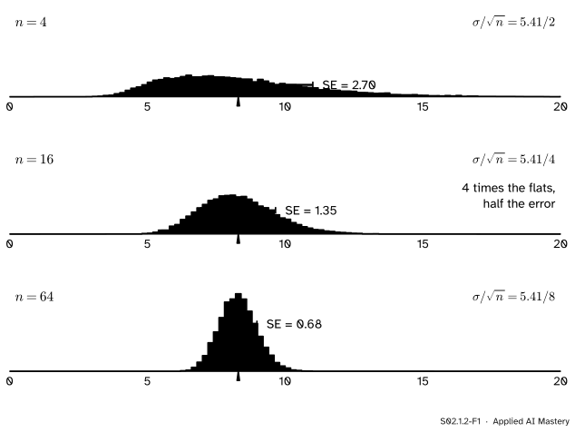
The last lesson drew the sampling distribution of \(\bar{x}\). Its width is the answer to the question: it says how far a sample mean typically lands from \(\mu\). Here it is for three sample sizes.
S02.1.2-F1
The sampling distribution of \(\bar{x}\) for samples of 4, 16 and 64 city rents. Each bar runs one standard error either side of \(\ctruth{\mu}\). Each time \(\cparam{n}\) is multiplied by four, the standard error halves.
The standard deviation of that pile has a name of its own, the standard error. It shrinks as \(n\) grows, but slowly: to halve it you need four times the data, and to cut it to a tenth you need a hundred times the data. Lesson S01.2.2 saw this happen in a simulation. This lesson proves it.
Build it up
Step 1. Name the width. The standard error of a statistic is the standard deviation of its sampling distribution. For the mean we write \(\operatorname{SE}(\bar{x})\).
Step 2. Recall the variance of a mean. For i.i.d. draws with variance \(\sigma^2\), lesson M06.11.1 showed that \({\operatorname{Var}(\bar{X})} = {\sigma^2 / n}\). The derivation is three lines:
The first line takes the constant \(1/n\) out of the variance as \(1/n^2\). The second uses independence: variances of independent variables add (M06.7). The third uses that every \(X_i\) has the same variance \(\sigma^2\).
Step 3. Take the square root. The standard error is the square root of that variance:
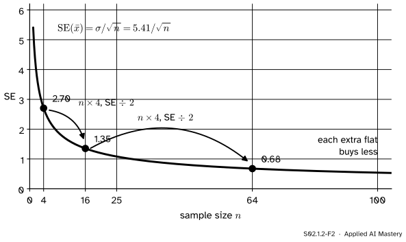
For the city, \(\sigma = 5.41\), so samples of 4, 16 and 64 have standard errors 2.70, 1.35 and 0.68.
Step 4. The square-root law. Multiply \(n\) by four and \(\sqrt{n}\) doubles, so the standard error halves. This is the law that S01.2.2 observed and promised to derive.
S02.1.2-F2
The standard error of the mean against \(n\). Each step from 4 to 16 to 64 multiplies \(n\) by four and halves the error. The curve flattens: each extra flat buys less precision than the one before.
Step 5. Estimate what you do not know. The formula needs \(\sigma\), which belongs to the population. From one sample we replace it with the sample standard deviation \(s\) (divisor \(n - 1\)), and get the estimated standard error
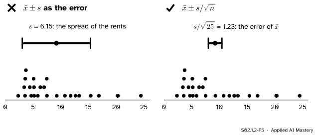
Your sample of 25 has \(s = 6.15\), so \(\widehat{\operatorname{se}} = {6.15 / 5} = 1.23\), close to the true 1.08. This is what software reports as “the standard error of the mean”.
The formal statement
NoteDefinition and results
The standard error of a statistic \(T\) is \({\operatorname{SE}(T)} = {\sqrt{\operatorname{Var}(T)}}\), the standard deviation of its sampling distribution.
The factor \((N - n)/(N - 1)\) in Result 2 is the finite population correction.
Result 2, derived. Draw \(n\) units one after another without replacement and call their values \(X_1, \dots, X_n\). Expand the variance of the sum into variances and covariances (M06.10):
Two symmetry facts fill it in. Each single draw is equally likely to be any of the \(N\) units, so \({\operatorname{Var}(X_i)} = \sigma^2\). Each pair of draws \((X_i, X_j)\) is equally likely to be any ordered pair of two different units, so every pair has the same covariance; call it \(c\). That pair is chosen the same way however many draws come after it, so \(c\) does not depend on \(n\). There are \(n\) variance terms and \(n(n - 1)\) ordered pairs:
To find \(c\), take \(n = N\). Then the sample is the whole population and the sum is the population total, the same number every time, so its variance is 0:
The last line puts \(1 - (n-1)/(N-1)\) over the common denominator \(N - 1\). Dividing by \(n^2\), because \(\bar{X}\) is the sum divided by \(n\), gives Result 2.
S02.1.2-F4
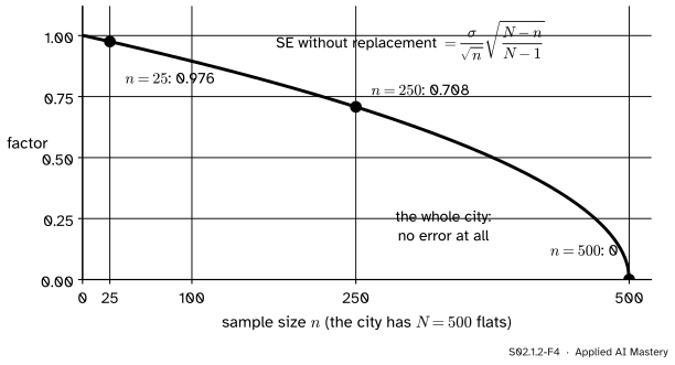
The finite population correction to the standard error, \(\sqrt{(N - n)/(N - 1)}\), for the city. For 25 flats it is 0.976, so it barely matters. It matters only when the sample is a large share of the population, and it reaches 0 when the sample is the whole city.
Result 3, derived. A proportion is a mean of 0s and 1s. Let \(X_i = 1\) if unit \(i\) has the property (a flat above 10, a test example answered correctly) and 0 if not, with \(P(X_i = 1) = p\). Then \(\hat{p} = \bar{X}\), and \(\E[X_i] = p\). Because \(X_i^2 = X_i\) for a 0 or 1, \(\E[X_i^2] = p\), so
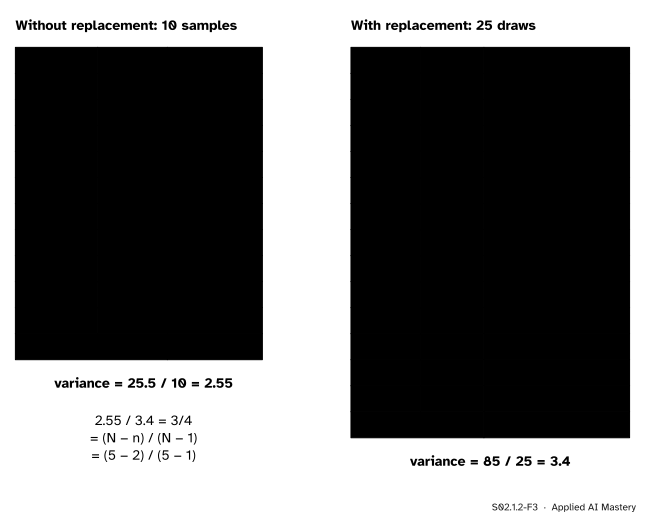
Samples of \(n = 2\). With replacement, Result 1 predicts \({\operatorname{Var}(\bar{X})} = {6.8 / 2} = 3.4\). Without, Result 2 predicts \({3.4 \times (5 - 2)/(5 - 1)} = {3.4 \times 3/4} = 2.55\). Now list every sample and compute the variances directly.
S02.1.2-F3
Both variances worked by listing every sample. Every sample mean averages 8, so each variance is the mean squared distance from 8. Their ratio is the finite population correction.
Without replacement. The ten samples have means 5.5, 6, 6.5, 8, 7.5, 8, 9.5, 8.5, 10 and 10.5. Their squared distances from 8 are 6.25, 4, 2.25, 0, 0.25, 0, 2.25, 0.25, 4 and 6.25, which add to 25.5. So \({\operatorname{Var}(\bar{X})} = {25.5 / 10} = 2.55\).
With replacement. Group the 25 ordered draws of the last lesson by their mean. The value 4 occurs once, at squared distance 16; the value 5.5 twice, at 6.25 each, adding 12.5; and so on down the table. The thirteen rows add to 85, so \({\operatorname{Var}(\bar{X})} = {85 / 25} = 3.4\).
The city at \(n = 25\). With replacement, \({\operatorname{SE}(\bar{x})} = {5.41 / \sqrt{25}} = 1.082\). Without, multiply by \({\sqrt{(500 - 25)/(500 - 1)}} = {\sqrt{475/499}} = 0.976\), which gives 1.056.
Code
From scratch: the formulas for the city, then a simulation of 20,000 samples of 25 each way.
import mathimport numpy as npfrom scipy import statsrng = np.random.default_rng(0)rents = []for size, district_mean in ((250, 5), (150, 8), (100, 17)): draws = rng.gamma(9.0, 1.0, size) rents.append(draws * district_mean / draws.mean())rents = np.concatenate(rents)N, n =len(rents), 25sigma = rents.std() # divisor Nse_with = sigma / math.sqrt(n)se_without = se_with * math.sqrt((N - n) / (N -1))print(f"formula: with {se_with:.3f}, without {se_without:.3f}")rng = np.random.default_rng(4)with_repl = rng.choice(rents, size=(20_000, n)).mean(axis=1)without = np.array([rng.choice(rents, n, replace=False).mean() for _ inrange(20_000)])print(f"simulated: with {with_repl.std():.3f}, without {without.std():.3f}")
formula: with 1.082, without 1.056
simulated: with 1.081, without 1.057
The simulated standard deviations, 1.081 and 1.057, agree with the formulas to within simulation noise. The five flats, listed exactly:
import itertoolsfive = np.array([4, 7, 8, 9, 12])var_pop = five.var() # divisor N: 6.8with2 = [(a + b) /2for a, b in itertools.product(five, repeat=2)]without2 = [(a + b) /2for a, b in itertools.combinations(five, 2)]print(var_pop, np.var(with2), np.var(without2), np.var(without2) / np.var(with2))
6.8 3.4 2.55 0.75
From one sample, the estimated standard error by hand and with scipy.stats.sem, whose ddof defaults to 1, so it divides by \(n - 1\) inside \(s\). Then a proportion: a classifier right on 90 of 100 test examples.
So 90 correct out of 100 has an estimated standard error of 0.03: the next test set of 100 could easily score 0.87 or 0.93.
Explore
The module’s interactive, in lesson S02.1.3, reports the standard deviation of the statistics you have drawn beside the theoretical \(\sigma/\sqrt{n}\). Try \(n = 4\) and then \(n = 16\) there, and watch the second number halve.
Pitfalls
S02.1.2-F5
Wrong beside right. The standard deviation \(s\) measures how single rents vary. The standard error \(s / \sqrt{n}\) measures how the mean varies. They differ by the factor \(\sqrt{25} = 5\).
“The standard deviation and the standard error are the same thing.”
The standard deviation describes the data: single rents scatter by about 6 around their mean, and more data will not change that. The standard error describes a statistic: means of 25 rents scatter by about 1.2, and more data shrinks it. Reporting \(\bar{x} \pm s\) as the uncertainty of a mean overstates it fivefold here.
“Twice the data, half the error.”
Twice the data divides the standard error by \(\sqrt{2} \approx 1.41\), not by 2. To halve it you need four times the data. A model evaluated on 10,000 test examples instead of 2,500 has half the standard error on its accuracy, not a quarter.
“A sample of 1,000 is useless in a country of 100 million: it is a tiny share.”
The standard error depends on \(n\), not on the share \(n/N\), unless that share is large. For 1,000 people from a city of 20,000 the correction is \({\sqrt{19{,}000 / 19{,}999}} \approx 0.975\); from a country it is practically 1. Both polls are about equally precise.
Check yourself
Recall
1. What is the standard error of a statistic?
Show answer
The standard deviation of its sampling distribution.
2. What is \(\operatorname{SE}(\bar{x})\) for i.i.d. draws, and what happens to it when \(n\) is multiplied by four?
Show answer
\(\sigma / \sqrt{n}\). It halves, because \(\sqrt{4n} = 2\sqrt{n}\).
3. What is the finite population correction, and what is it for 25 flats out of 500?
Show answer
The factor \((N - n)/(N - 1)\) on the variance of \(\bar{X}\) without replacement. For the city it is \(475/499\), which multiplies the standard error by \(\sqrt{475/499} = 0.976\).
4. Why is the covariance of two draws without replacement negative?
Show answer
Because the population total is fixed: a high first draw leaves lower values for the second. Taking \(n = N\) forces \(c = -\sigma^2/(N - 1)\).
5. What is the estimated standard error of an accuracy of 0.9 on 100 test examples?
Show answer
\({\sqrt{0.9 \times 0.1 / 100}} = 0.03\).
Exercises
1.★ A share 0.254 of the city’s flats rent above 10. Find the standard error of the share \(\hat{p}\) above 10 in a sample of 25 drawn with replacement, and in a sample of 100.
Show solution
\({\sqrt{0.254 \times 0.746 / 25}} = {\sqrt{0.0075794}} = 0.087\). For \(n = 100\) it is half that, \(0.0435\), because the sample is four times larger.
2.★★ Draw \(n = 3\) of the five flats without replacement. Use Result 2 to predict \(\operatorname{Var}(\bar{X})\), then check it by listing the ten samples.
Listing: the ten samples of three have sums 19, 20, 23, 21, 24, 25, 24, 27, 28 and 29 (from \(\{4,7,8\}\), \(\{4,7,9\}\), \(\{4,7,12\}\), \(\{4,8,9\}\), \(\{4,8,12\}\), \(\{4,9,12\}\), \(\{7,8,9\}\), \(\{7,8,12\}\), \(\{7,9,12\}\) and \(\{8,9,12\}\)). Each mean is the sum divided by 3, and the mean of the means is 8, so each squared distance is (sum − 24)² / 9. The sums minus 24 are −5, −4, −1, −3, 0, 1, 0, 3, 4 and 5, whose squares add to 102. So \({\operatorname{Var}(\bar{X})} = {102 / (9 \times 10)} = 1.1333\), as predicted.
3.★★★ Show from Result 2 that sampling without replacement never has a larger variance than sampling with replacement, and that the two agree when \(n = 1\). Then explain why the derivation needed \(c\) to be the same for every \(n\).
Show solution
The ratio of the two variances is \((N - n)/(N - 1)\). For \(1 \le n \le N\) the numerator is at most the denominator, because \(N - n \le N - 1\) exactly when \(n \ge 1\), so the ratio is at most 1; it equals 1 at \(n = 1\), where one draw cannot depend on another. The value of \(c\) was found by setting \(n = N\) and then used for a smaller \(n\). That step is valid only because the first two draws of a sample are chosen the same way whatever the sample size: the pair \((X_1, X_2)\) is a uniformly random ordered pair of distinct units whether \(n = 2\) or \(n = N\).
Summary card
The standard error is the width of the sampling distribution.
S02.1.2-F1
Four times the data, half the error.
\({\operatorname{SE}(\bar{x})} = {\sigma/\sqrt{n}}\); estimated by \(s/\sqrt{n}\) (scipy.stats.sem).
Without replacement: multiply the variance by \((N - n)/(N - 1)\).
Proportion: \({\operatorname{SE}(\hat{p})} = {\sqrt{p(1 - p)/n}}\); 0.03 for 0.9 on 100 examples.
City, \(n = 25\): 1.082 with replacement, 1.056 without.
Sources and next steps
Sources. Each was opened and checked against this lesson on 15 November 2026.
Konstantin Zuev, Math 408 Mathematical Statistics, Lecture 15: accuracy of estimation of the population mean (2013). It defines the population variance with divisor \(N\) and gives the Lemma that \({\operatorname{Cov}(X_i, X_j)} = {-\sigma^2/(N - 1)}\) for \(i \ne j\) under simple random sampling; the Theorem giving \(\operatorname{Var}(\bar{X}_n)\) as \(\sigma^2/n\) times \({1 - (n-1)/(N-1)}\), a factor it names the finite population correction; and the remark that doubling the accuracy needs four times the sample.
David Diez, Mine Cetinkaya-Rundel and Christopher Barr, OpenIntro Statistics, 4th edition. Section 5.1.2 calls the standard deviation of a sampling distribution its standard error; Section 5.1.3 gives \(\operatorname{SE}_{\hat{p}} = {\sqrt{p(1 - p)/n}}\) and, in a footnote, the correction factor \(\sqrt{(N - n)/(N - 1)}\), small when \(n < 0.1N\).
SciPy reference, scipy.stats.sem: the signature sem(a, axis=0, ddof=1, ...), and the note that its default ddof=1 differs from the 0 of other routines.