Treat the right-hand side of a Bellman equation as a machine that turns any table of values into a new one. Prove that both machines pull any two tables closer by the discount factor, and see why repeating a backup converges to the right values from any starting guess.
Apply the expectation backup and the max backup to an arbitrary table of values, by hand and in code.
State what it means for a table to be a fixed point of a backup, and name the fixed point of each.
Prove that both backups are contractions in the max norm with factor equal to the discount rate.
Use the contraction property to bound the error after a given number of sweeps and to show that the fixed point is unique.
In review. The maths and code on this page are checked by automated tests on every change, but an independent reader has not signed it off yet. Spot a mistake or a confusing step? Tell us.
The question
The lake has two states, so its Bellman equations can be solved by hand. A real problem has thousands of states, or millions. Suppose we just guess a value for every state, feed the guesses into the right-hand side of the equation, and repeat. Why should the numbers ever settle, and why on the right answer?
From the last lesson
1. State the Bellman optimality equation for \(v_*\).
Show answer
\(v_*(s) = \max_a \sum_{s', r} p(s', r \mid s, a)\,[\,r + \gamma\, v_*(s')\,]\), for every state \(s\).
2. Why can the optimal values not be found by one linear solve?
Show answer
Because of the maximum. A maximum of linear expressions is not linear, so the optimality equations are not a linear system.
Intuition
Look at the right-hand side of a Bellman equation on its own. It takes a value for every state and returns one for every state. It is a machine: a table of values goes in, a new table comes out. Such a machine is an operator, and one use of it is a backup.
RL01.6.4-F1
One backup in a small gridworld: \(T_*\) recomputes every cell of the left-hand table from its neighbours’ old values and returns the table on the right.
Two ideas make it useful.
Fixed points. A table that comes out exactly as it went in is a fixed point. The Bellman equations say that the true values are fixed points: \(v_\pi\) of one machine, \(v_*\) of the other.
Contraction. Feed the machine two tables and the results are closer together than the tables were. So any guess is pulled towards the fixed point, sweep after sweep.
Build it up
Step 1. A table is just numbers. It gives one number to each state, and need not be the value function of any policy. For the lake, a table is a pair: a point in the plane.
Step 2. Two backups. The expectation backup\(T_\pi\) applies the right-hand side of the Bellman expectation equation for a policy \(\pi\). The max backup\(T_*\) applies the right-hand side of the Bellman optimality equation.
Step 3. A distance between tables. Two tables are close if they are close in every state. Their distance is the largest gap between them in any state.
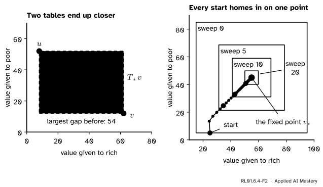
Step 4. One backup shrinks the distance. Take the lake tables \(u = (8, 52)\) and \(v = (62, 12)\), in the order (rich, poor). Their largest gap is 54. The max backup turns them into \((37, 47.8)\) and \((57.8, 33.3)\), whose largest gap is 20.8.
RL01.6.4-F2
The lake’s tables as points. Left: one max backup moves two tables closer: the largest gap falls from 54 to 20.8, well under \(0.9 \times 54\). Right: repeated backups from \((25, 5)\). After \(k\) sweeps the table must lie in a square around \(v_*\) whose side has shrunk by \(0.9^k\).
Step 5. Repeat. Let one of the two tables be the fixed point. It does not move, so the other gets closer to it with every sweep, whatever the starting guess.
The formal statement
Throughout, the states are the non-terminal ones, a table\(v\) gives a real number \(v(s)\) to each, and terminal states count as value 0.
NoteDefinitions: the Bellman operators and the max norm
For any table \(v\), the two backups produce the tables \(T_\pi v\) and \(T_* v\) with entries
\[
\begin{aligned}
& (T_\pi v)(s) \\
&\quad = \sum_{a} \pi(a \mid s) \sum_{s', r} p(s', r \mid s, a) \\
&\qquad\quad \times\; \big[ r + \gamma v(s') \big], \\
& (T_* v)(s) \\
&\quad = \max_{a} \sum_{s', r} p(s', r \mid s, a) \\
&\qquad\quad \times\; \big[ r + \gamma v(s') \big] .
\end{aligned}
\]
The distance between two tables is the max norm of their difference: \(\norm{u - v}_\infty = \max_s \abs{u(s) - v(s)}\).
The two Bellman equations are now one line each: \(T_\pi v_\pi = v_\pi\) and \(T_* v_* = v_*\).
NoteTheorem: both backups are contractions
For all tables \(u\) and \(v\), and for \(T\) equal to \(T_\pi\) or to \(T_*\),
\[
\norm{T u - T v}_\infty \;\le\; \cparam{\gamma}\; \norm{u - v}_\infty .
\]
Proof for \(T_\pi\). Fix a state \(s\) and subtract. The rewards cancel:
Take absolute values. The weights \(\pi(a \mid s)\, p(s', r \mid s, a)\) are never negative, so the absolute value of the weighted sum is at most the weighted sum of absolute values. Each \(\abs{u(s') - v(s')}\) is at most \(\norm{u - v}_\infty\), and the weights sum to 1:
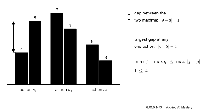
So \(\max f - \max g \le \max \abs{f - g}\). Swap the roles of \(f\) and \(g\) to get \(\max g - \max f \le \max \abs{f - g}\). A number and its negative are both at most \(\max \abs{f - g}\), so its absolute value is too. \(\blacksquare\)
Proof for \(T_*\). Fix a state \(s\). Let \(f(a)\) be the look-ahead for action \(a\) computed with the table \(u\), and \(g(a)\) the same with \(v\). Then \((T_* u)(s) = \max_a f(a)\) and \((T_* v)(s) = \max_a g(a)\), and the lemma gives
For each single action, \(f(a) - g(a) = \gamma \sum_{s', r} p(s', r \mid s, a)\,[\,u(s') - v(s')\,]\), and the argument used for \(T_\pi\) shows that this is at most \(\gamma\, \norm{u - v}_\infty\) in absolute value. So the same bound holds in every state. \(\blacksquare\)
Four consequences. Let \(T\) be either backup and \(\bar v\) its fixed point (\(v_\pi\) or \(v_*\)). Start from any table \(v_0\) and sweep: \(v_{k+1} = T v_k\).
The error shrinks. Since \(T \bar v = \bar v\), \(\norm{v_{k+1} - \bar v}_\infty = \norm{T v_k - T \bar v}_\infty \le \gamma\, \norm{v_k - \bar v}_\infty\). Applying this \(k\) times, \(\norm{v_k - \bar v}_\infty \le \gamma^k\, \norm{v_0 - \bar v}_\infty\), which goes to 0 when \(\gamma < 1\).
The fixed point is unique. If \(w\) is also a fixed point, then \(\norm{w - \bar v}_\infty = \norm{T w - T \bar v}_\infty \le \gamma\, \norm{w - \bar v}_\infty\). With \(\gamma < 1\) that forces \(\norm{w - \bar v}_\infty = 0\), so \(w = \bar v\). Each Bellman equation has exactly one solution.
The change per sweep shrinks.\(\norm{v_{k+1} - v_k}_\infty = \norm{T v_k - T v_{k-1}}_\infty \le \gamma\, \norm{v_k - v_{k-1}}_\infty\). This can be watched without knowing \(\bar v\).
A stopping rule. By the triangle inequality and consequence 1, \(\norm{v_k - \bar v}_\infty \le \norm{v_k - v_{k+1}}_\infty + \gamma\, \norm{v_k - \bar v}_\infty\). So \(\norm{v_k - \bar v}_\infty \le \norm{v_{k+1} - v_k}_\infty / (1 - \gamma)\), and after one more sweep \(\norm{v_{k+1} - \bar v}_\infty \le \tfrac{\gamma}{1 - \gamma}\, \norm{v_{k+1} - v_k}_\infty\).
Sweeping with \(T_\pi\) is iterative policy evaluation (module RL01.7). Sweeping with \(T_*\) is value iteration (module RL01.8).
Go deeper: why the max backup has a fixed point, and why it is the optimal value
The last lesson borrowed two facts to show that \(v_*\) solves the optimality equation. The contraction property needs neither. Take \(\gamma < 1\).
A fixed point exists. Sweep from any \(v_0\). By consequence 3, \(\norm{v_{k+1} - v_k}_\infty \le \gamma^k \norm{v_1 - v_0}_\infty\). For \(m > k\), the triangle inequality and a geometric series give \(\norm{v_m - v_k}_\infty \le \tfrac{\gamma^k}{1 - \gamma}\norm{v_1 - v_0}_\infty\), which is as small as we like for large \(k\). So in each state \(v_k(s)\) is a Cauchy sequence, with a limit \(V(s)\). Since \(\norm{T_* v_k - T_* V}_\infty \le \gamma \norm{v_k - V}_\infty \to 0\), letting \(k\) grow in \(v_{k+1} = T_* v_k\) gives \(V = T_* V\). This is Banach’s fixed-point theorem. By consequences 1 and 2, \(V\) is the only fixed point, and every start converges to it.
It is \(v_*\). An average never exceeds a maximum, so \(T_\pi v \le T_* v\) in every state. And \(T_*\) keeps order: if \(u \le v\) in every state, then \(T_* u \le T_* v\) (exercise 3a). So for any policy, \(v_\pi = T_\pi v_\pi \le T_* v_\pi \le T_*^2 v_\pi \le \cdots\), and this sequence converges to \(V\). Hence \(v_\pi \le V\) for every policy. Now let \(\pi\) be greedy with respect to \(V\). Then \(T_\pi V = T_* V = V\), so \(V\) is the fixed point of \(T_\pi\), which is \(v_\pi\). So \(V\) is the value of a policy that no policy beats: \(V = v_*\), and \(\pi\) is optimal.
The two links. The last lesson’s proof of Link 1 needed only an optimal policy, which now exists. And \(v_* = T_* v_*\), read with Link 1, is Link 2: \(v_*(s) = \max_a q_*(s, a)\).
Worked example
Sweep the max backup on the lake, starting from zeros. Tables are written (rich, poor); \(\gamma = 0.9\). Each entry is the larger of the rod’s look-ahead and the net’s.
Compare each \(v_k\) with \(v_* = (55, 45)\): its distance, and the bound \(0.9^k \times 55\).
\(k\)
\(v_k\)
Distance
Bound
0
(0, 0)
55
55
1
(10, 1)
45
49.5
2
(14.95, 4.95)
40.05
44.55
3
(18.955, 8.955)
36.045
40.095
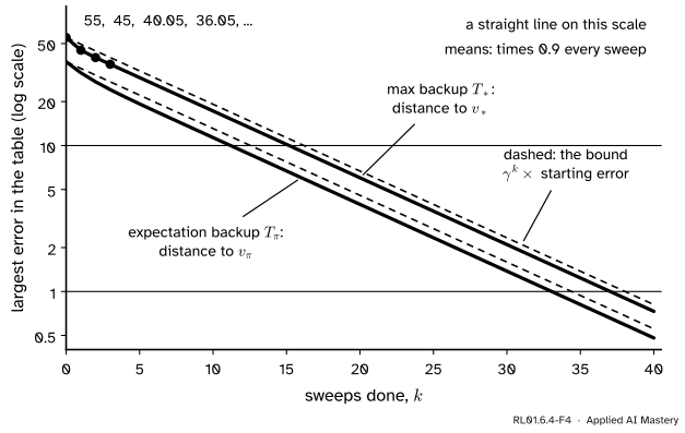
The distance stays under the bound of consequence 1. From sweep 2 to sweep 3 it is multiplied by exactly 0.9, so the factor \(\gamma\) in the theorem cannot be improved.
RL01.6.4-F4
Forty sweeps of each backup on the lake, from zeros. Each solid line stays below its dashed bound.
The stopping rule is just as sharp. The last sweep changed the table by \(\norm{v_3 - v_2}_\infty = 4.005\), and the true error of \(v_3\) is \(36.045 = 9 \times 4.005\): the full factor \(\gamma / (1 - \gamma) = 9\) of consequence 4.
The expectation backup behaves the same way. For the coin-toss policy of lesson RL01.6.2, sweeping from zeros gives \(v_1 = (6, 0.5)\) and \(v_2 = (10.1625,\ 2.1875)\). Their distances to \(v_\pi = (37.5, 27.5)\) are 31.5 and 27.3375, under the bounds \(0.9 \times 37.5 = 33.75\) and \(0.81 \times 37.5 = 30.375\).
Code
Both backups from scratch, on the lake.
GAMMA =0.9STATES = ["rich", "poor"]ACTIONS = ["rod", "net"]p = { # p[(state, action)] lists the outcomes as (probability, next state, reward) ("rich", "rod"): [(1.0, "rich", 2)], ("rich", "net"): [(0.5, "rich", 10), (0.5, "poor", 10)], ("poor", "rod"): [(0.5, "rich", 0), (0.5, "poor", 0)], ("poor", "net"): [(1.0, "poor", 1)],}coin_toss = {s: {"rod": 0.5, "net": 0.5} for s in STATES}def look_ahead(v, s, a):returnsum(prob * (r + GAMMA * v[s2]) for prob, s2, r in p[(s, a)])def T_pi(v, pi=coin_toss):"""The expectation backup: average the look-aheads with the policy's probabilities."""return {s: sum(pi[s][a] * look_ahead(v, s, a) for a in ACTIONS) for s in STATES}def T_star(v):"""The max backup: keep the best look-ahead."""return {s: max(look_ahead(v, s, a) for a in ACTIONS) for s in STATES}def distance(u, v):"""The max norm of u - v: the largest gap in any state."""returnmax(abs(u[s] - v[s]) for s in STATES)def sweeps(T, target, count): v = {s: 0.0for s in STATES} errors = [distance(v, target)]for _ inrange(count): v = T(v) errors.append(distance(v, target))return v, errorsv_pi, v_star = {"rich": 37.5, "poor": 27.5}, {"rich": 55.0, "poor": 45.0}end_pi, err_pi = sweeps(T_pi, v_pi, 300)end_star, err_star = sweeps(T_star, v_star, 300)for name, errors in (("max backup", err_star), ("expectation backup", err_pi)):print(name)print(" k error ratio")for k inrange(1, 6):print(f"{k:>3}{errors[k]:8.4f}{errors[k] / errors[k -1]:.4f}")print("max backup, 300 sweeps:", [round(x, 6) for x in end_star.values()])print("expectation, 300 sweeps:", [round(x, 6) for x in end_pi.values()])
max backup
  k    error  ratio
  1  45.0000 0.8182
  2  40.0500 0.8900
  3  36.0450 0.9000
  4  32.4405 0.9000
  5  29.1964 0.9000
expectation backup
  k    error  ratio
  1  31.5000 0.8400
  2  27.3375 0.8679
  3  24.1481 0.8833
  4  21.5283 0.8915
  5  19.2832 0.8957
max backup, 300 sweeps: [55.0, 45.0]
expectation, 300 sweeps: [37.5, 27.5]
No ratio exceeds 0.9, and both runs end at the hand-found values. The theorem covers any two tables, so test it and the lemma on random inputs.
import numpy as nprng = np.random.default_rng(0)worst = {"T_pi": 0.0, "T_star": 0.0}for _ inrange(2000): u =dict(zip(STATES, rng.uniform(-100, 100, size=2))) v =dict(zip(STATES, rng.uniform(-100, 100, size=2))) worst["T_pi"] =max(worst["T_pi"], distance(T_pi(u), T_pi(v)) / distance(u, v)) worst["T_star"] =max(worst["T_star"], distance(T_star(u), T_star(v)) / distance(u, v))for name, x in worst.items():print(f"largest shrink factor, {name}: {float(x):.4f}")f, g = rng.normal(size=(2000, 4)), rng.normal(size=(2000, 4))gap_of_maxima = np.abs(f.max(axis=1) - g.max(axis=1))largest_gap = np.abs(f - g).max(axis=1)lemma_holds =bool(np.all(gap_of_maxima <= largest_gap +1e-12))print("lemma holds on 2000 lists:", lemma_holds)
largest shrink factor, T_pi: 0.8999
largest shrink factor, T_star: 0.9000
lemma holds on 2000 lists: True
With NumPy the expectation backup is one line, \(\vect{r}_\pi + \gamma\, \mat{P}_\pi \vect{v}\). Repeating it reaches the np.linalg.solve answer of lesson RL01.6.2.
repeated backup: [37.5 27.5]
direct solve:    [37.5 27.5]
A sweep costs a few multiplications per state and outcome; the direct solve costs the cube of the number of states. So large problems are swept, not solved.
Explore
RL01.6-X1
Bellman backup gridworld
Press One sweep and watch values spread out from the goal and the pit, one cell per sweep. Select a cell to see its backup written out, then switch between the max and the average.
The rules of this gridworld, in the interactive and the figures:
The grid has four columns and three rows; one cell is a wall. The goal and the pit are terminal, so their value is fixed at 0.
The agent chooses up, right, down or left. With probability \(1 - \text{slip}\) the move goes where intended. Otherwise it goes sideways: a quarter turn to either side, each with probability \(\text{slip} / 2\).
A move into the wall or off the edge leaves the agent where it is.
The reward is \(+1\) for entering the goal, \(-1\) for entering the pit, and the reward per step for every other move, including a blocked one.
A sweep is synchronous: every new value comes from the old table. An arrowhead marks each greedy move; a cell shows none while all four moves tie.
Things to try, with the starting settings \(\gamma = 0.9\), slip 0.2 and reward per step \(-0.04\):
Before any sweep, select the cell left of the goal. Its entry for “right” is \(0.8 \times (1 + 0.9 \times 0)\) plus two slips of \(0.1 \times (-0.04 + 0.9 \times 0)\): 0.79 in all. After one sweep that cell shows 0.79 and every other cell \(-0.04\).
Press Run. The max backup settles at 0.93 left of the goal and 0.37 in the bottom-left corner, and each sweep multiplies the read-out’s largest change by at most \(\gamma\). With the random policy the same two cells settle at 0.10 and \(-0.40\).
Return to the max backup with \(\gamma = 0.99\) and a reward per step of \(+0.1\), reset and run. Staying on the grid now pays, so the arrows turn away from the goal, and the run takes about 750 sweeps where the starting settings took 16.
Pitfalls
RL01.6.4-F5
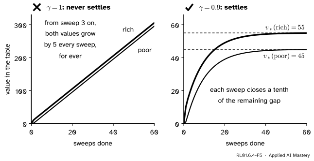
Wrong beside right. With \(\gamma = 1\) the theorem promises no shrinking, and the lake’s sweeps never settle. With \(\gamma = 0.9\) they settle at \(v_*\).
“Sweeping always converges.”
The proof needs \(\gamma < 1\). With \(\gamma = 1\) the bound only says “no further apart”. The lake never ends and pays 5 fish a day on average under the best plan, so its undiscounted values are infinite and the table grows for ever. Without discounting, Sutton and Barto guarantee \(v_\pi\) only when the policy is certain to end the task, which this proof does not cover.
“The last sweep changed nothing much, so the table is accurate.”
The error can be \(\gamma / (1 - \gamma)\) times larger than the change. With \(\gamma = 0.9\) that is 9 times, as in the worked example, and with \(\gamma = 0.99\) it is 99 times. When a learning system is stopped “at convergence”, choose the threshold from consequence 4, not by eye.
“A contraction improves every entry of the table on every sweep.”
Only the largest error is certain to shrink. Start the lake at \((55, 0)\): the rich entry is exact and the poor entry is off by 45. One max backup gives \((51.5, 24.75)\). The largest error fell to 20.25, but the rich entry is now off by 3.5.
Check yourself
Recall
1. What does a Bellman operator take in, and what does it give back?
Show answer
It takes a table with one value per state and gives back a new table of the same shape, computed with the right-hand side of a Bellman equation.
2. What is a fixed point of an operator \(T\), and what are the fixed points of \(T_\pi\) and \(T_*\)?
Show answer
A table \(v\) with \(T v = v\). The fixed point of \(T_\pi\) is \(v_\pi\) and the fixed point of \(T_*\) is \(v_*\).
3. How is the distance between two tables measured in this lesson?
Show answer
By the max norm: the largest absolute difference between them in any single state.
4. State the contraction property of the two backups.
Show answer
\(\norm{T u - T v}_\infty \le \gamma\, \norm{u - v}_\infty\) for all tables \(u\) and \(v\): one backup shrinks the distance between any two tables by at least the factor \(\gamma\).
5. After \(k\) sweeps from a table \(v_0\), how far can the table be from the fixed point?
Show answer
At most \(\gamma^k\) times the starting distance: \(\norm{v_k - \bar v}_\infty \le \gamma^k \norm{v_0 - \bar v}_\infty\).
Exercises
1.★ Apply the expectation backup of the coin-toss policy once to the lake table \(v = (10, 0)\), written (rich, poor).
Show solution
Use \(T_\pi v = (6 + 0.675\,v(\text{rich}) + 0.225\,v(\text{poor}),\; 0.5 + 0.225\,v(\text{rich}) + 0.675\,v(\text{poor}))\). Rich: \(6 + 0.675 \times 10 + 0 = 12.75\). Poor: \(0.5 + 0.225 \times 10 + 0 = 2.75\). So \(T_\pi v = (12.75,\ 2.75)\).
2.★★ Value iteration on the lake starts from zeros, a distance of 55 from \(v_*\). How many sweeps guarantee that every entry is within 0.01 of \(v_*\)?
Show solution
By consequence 1 the error after \(k\) sweeps is at most \(0.9^k \times 55\). We need \(0.9^k \times 55 < 0.01\), that is \(0.9^k < 0.01 / 55\). Taking logarithms, \(k > \ln(5500) / \ln(1 / 0.9) = 8.6125 / 0.10536 \approx 81.7\). So 82 sweeps are enough: \(0.9^{82} \times 55 \approx 0.0097\), while \(0.9^{81} \times 55 \approx 0.0108\).
3.★★★ Prove the contraction property of \(T_*\) again without the lemma, from two simpler facts. (a) Monotone: if \(u(s) \le v(s)\) in every state, then \((T_* u)(s) \le (T_* v)(s)\) in every state. (b) Shift: adding a constant \(c\) to every entry of \(v\) adds \(\gamma c\) to every entry of \(T_* v\). Assume no terminal states.
Show solution
(a) Each look-ahead \(\sum p\,[\,r + \gamma u(s')\,]\) puts non-negative weights \(\gamma p\) on the entries of \(u\), so raising entries cannot lower it. If every look-ahead with \(v\) is at least the one with \(u\), so is the maximum.
(b) The look-ahead with \(v + c\) is \(\sum p\,[\,r + \gamma v(s') + \gamma c\,]\): the look-ahead with \(v\) plus \(\gamma c\), because the probabilities sum to 1. Adding one number to every look-ahead adds it to the maximum.
Now let \(d = \norm{u - v}_\infty\), so \(u(s) \le v(s) + d\) in every state. By (a) and then (b), \(T_* u \le T_*(v + d) = T_* v + \gamma d\). Swapping \(u\) and \(v\) gives \(T_* v \le T_* u + \gamma d\). Together, \(\abs{(T_* u)(s) - (T_* v)(s)} \le \gamma d\) in every state: the contraction property. The same proof works for \(T_\pi\).
Summary card
A backup turns a table of values into a better one, and repeating it converges, because each sweep multiplies the largest error by at most \(\gamma\).
RL01.6.4-F1
Table in, table out.
Operators.\((T_\pi v)(s) = \sum_a \pi(a \mid s) \sum_{s', r} p(s', r \mid s, a)\,[\,r + \gamma v(s')\,]\), and \(T_*\) has \(\max_a\) in place of the average.
Fixed points.\(T_\pi v_\pi = v_\pi\) and \(T_* v_* = v_*\), and each is the only one.
Contraction.\(\norm{T u - T v}_\infty \le \gamma\, \norm{u - v}_\infty\) for both backups.
Convergence.\(\norm{v_k - \bar v}_\infty \le \gamma^k\, \norm{v_0 - \bar v}_\infty\) from any start.
Sources. Each was opened and checked against this lesson on 12 November 2026.
Csaba Szepesvári, Algorithms for Reinforcement Learning, the author’s draft. Section 2.3 defines the Bellman operator of a policy and the Bellman optimality operator, equation (13), and states that both are max-norm contractions when \(0 < \gamma < 1\). Appendix A proves Banach’s fixed-point theorem with the rate \(\gamma^n\) (Theorem 1), both contractions, the second with the inequality on maxima, and that the fixed point is the optimal value (Theorem 2).
David Silver, Reinforcement Learning, lecture course (Advanced Topics 2015), Lecture 3: Planning by Dynamic Programming. The closing section “Contraction Mapping” uses the ∞-norm, shows that the Bellman expectation backup is a \(\gamma\)-contraction, and concludes that iterative policy evaluation and value iteration converge.
Richard S. Sutton and Andrew G. Barto, Reinforcement Learning: An Introduction, 2nd edition, MIT Press, 2018. Section 4.1 guarantees \(v_\pi\) when \(\gamma < 1\) or the policy is certain to terminate, and gives iterative policy evaluation as update (4.5), stopped by the largest change in a sweep. Section 4.4 gives value iteration as update (4.10).
Next. Modules RL01.7, Policy evaluation, and RL01.8, Policy iteration and value iteration, turn the two backups into algorithms.