Replace the average over actions by a maximum and the Bellman equation describes the best possible behaviour instead of a given one. Meet the optimal value functions, see why acting greedily on them is optimal, and find the best policy of a small problem by checking every candidate.
State the Bellman optimality equations for the optimal state values and the optimal action values.
Explain why a policy that is greedy with respect to the optimal values is an optimal policy.
Find the optimal policy of a small Markov decision process by evaluating every deterministic policy, and verify the result with the optimality equation.
Explain why the maximum makes the equations non-linear, so that no single linear solve finds the optimal values.
Say precisely what acting greedily on the values of an arbitrary policy does and does not guarantee.
In review. The maths and code on this page are checked by automated tests on every change, but an independent reader has not signed it off yet. Spot a mistake or a confusing step? Tell us.
The question
At a poor lake the net catches one fish today and the rod catches none. Yet the best fisher reaches for the rod. Which action is best in each state, what is each state worth when the fisher always acts for the best, and can we find out without trying every possible plan?
From the last lesson
1. State the Bellman expectation equation for \(v_\pi\).
Show answer
\(v_\pi(s) = \sum_a \pi(a \mid s) \sum_{s', r} p(s', r \mid s, a)\,[\,r + \gamma\, v_\pi(s')\,]\), for every state \(s\).
2. How do you get \(v_\pi(s)\) from the action values \(q_\pi(s, a)\)?
Show answer
Average them with the policy’s probabilities: \(v_\pi(s) = \sum_a \pi(a \mid s)\, q_\pi(s, a)\).
Intuition
The last lesson asked what a state is worth under a given policy. This lesson asks what it is worth under the best policy. Write \(v_*(s)\) for that best possible value.
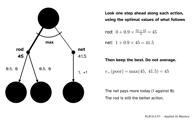
Suppose the best values of the next states were already known. Then choosing is easy. Look one step ahead along each action: its reward, plus \(\gamma\) times the average best value of where it leads. An agent that acts for the best takes the action with the largest result, and the state is worth exactly that result.
RL01.6.3-F1
The backup diagram for an optimal value, drawn for the poor lake. The only change from the last lesson is at the top: the arc says take the maximum over the actions where the policy’s average used to be. The best values 55 and 45 come from the worked example.
So the rule of the module, value now = reward + discount × value next, has two versions. Average over the actions and you get the value of a policy. Take the best action and you get the value of the best policy.
Build it up
Step 1. Say what “best” means. A policy \(\pi\) is at least as good as a policy \(\pi'\) if \(v_\pi(s) \ge v_{\pi'}(s)\) in every state \(s\). An optimal policy is at least as good as every other policy.
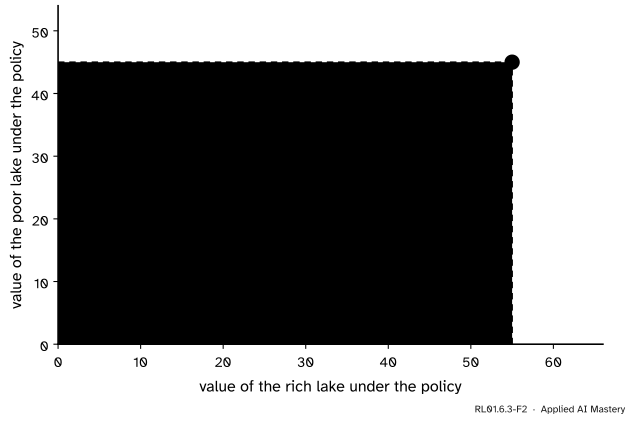
Step 2. Try every plan. The lake has two states and two actions, so there are four deterministic policies: plans that name one action for each state. Evaluate each with the method of the last lesson, and plot it as a point: its value at the rich lake across, its value at the poor lake up.
RL01.6.3-F2
Each policy of the lake is a point. One point lies above and to the right of all the others: the plan “net when rich, rod when poor” is best in both states at once.
Step 3. Name its values. The values at that point are the optimal values: \(v_*(\text{rich}) = 55\) and \(v_*(\text{poor}) = 45\).
Step 4. Spot the pattern. In each state the best plan takes the action with the largest one-step look-ahead, computed with the optimal values themselves. Written out for every state, that is the Bellman optimality equation.
Step 5. Use it to act. An agent that knows \(v_*\) can act by looking one step ahead and taking the best action.
The formal statement
NoteDefinitions: optimal value functions
The optimal state-value function and the optimal action-value function give the best value that any policy achieves:
\[
\begin{aligned}
v_*(s) &= \max_{\pi} v_\pi(s), \\
q_*(s, a) &= \max_{\pi} q_\pi(s, a) .
\end{aligned}
\]
A finite Markov decision process always has at least one optimal policy, and all optimal policies share these two functions (Sutton and Barto, Section 3.6). We take that as given here.
Compare the first line with the Bellman expectation equation. The environment, the discount and the values are where they were. The policy’s average\(\sum_a \pi(a \mid s)\) has become \(\max_a\). No policy appears at all.
Where the equations come from. Two links connect \(v_*\) and \(q_*\).
Link 1.\(q_*(s, a)\) is the best return available after taking \(a\) in \(s\). The first step pays \(r\) and lands in \(s'\), and the best that can be done from \(s'\) is \(v_*(s')\). Averaging over the outcomes,
\[
\begin{aligned}
q_*(s, a) = {} & \sum_{s', r} p(s', r \mid s, a) \\
& \times \big[ r + \gamma\, v_*(s') \big] .
\end{aligned}
\]
Link 2. The best value of a state is the value of its best first action:
\[
v_*(s) = \max_{a}\, q_*(s, a) .
\]
Put Link 1 into Link 2 and the equation for \(v_*\) appears. Put Link 2 into Link 1 and the equation for \(q_*\) appears: (3.19) and (3.20) in Sutton and Barto.
Go deeper: a proof of the two links
The proof uses two facts from Sutton and Barto: an optimal policy \(\pi_*\) exists (Section 3.6), and the policy improvement theorem (Section 4.2): if \(\pi'\) is a deterministic policy with \(q_\pi(s, \pi'(s)) \ge v_\pi(s)\) in every state, then \(v_{\pi'}(s) \ge v_\pi(s)\) in every state. It holds for a stochastic \(\pi\) too, as that section notes. Module RL01.8 proves the theorem. The next lesson gives a second route to the same links that needs neither fact.
Link 1. For any policy, \(q_\pi(s, a) = \sum_{s', r} p(s', r \mid s, a)\,[\,r + \gamma\, v_\pi(s')\,]\). Since \(v_\pi(s') \le v_*(s')\), this is at most \(\sum_{s', r} p(s', r \mid s, a)\,[\,r + \gamma\, v_*(s')\,]\), and \(\pi_*\) reaches that bound because \(v_{\pi_*} = v_*\). So the bound is the maximum over policies, \(q_*(s, a)\), and \(q_{\pi_*} = q_*\).
Link 2. Let \(\pi'\) pick, in each state, an action that maximises \(q_*(s, a)\). A maximum is never below a weighted average, so
By the theorem, \(v_{\pi'} \ge v_{\pi_*} = v_*\). No policy beats \(v_*\), so \(v_{\pi'} = v_*\). The value of a state under a deterministic policy is the action value of the action it takes, so
The third equality is Link 1, and the last holds by the choice of \(\pi'\).
Greedy policies. Given any table of values \(v\), a policy is greedy with respect to\(v\) if in every state it takes an action that maximises the one-step look-ahead \(\sum_{s', r} p(s', r \mid s, a)\,[\,r + \gamma\, v(s')\,]\).
NoteGreedy on the optimal values is optimal
When \(\gamma < 1\), every policy that is greedy with respect to \(v_*\) is an optimal policy.
Why. Let \(\pi\) be greedy with respect to \(v_*\) and deterministic. In every state its action attains the maximum in the optimality equation, so
Read this as a statement about \(\pi\): the table \(v_*\) satisfies the Bellman expectation equation of \(\pi\). The last lesson showed that, for \(\gamma < 1\), this equation has exactly one solution, \(v_\pi\). Hence \(v_\pi = v_*\), and \(\pi\) is optimal. The same argument covers a greedy policy that splits its probability among several maximising actions.
With \(q_*\) the agent needs even less. By Link 2, the best action in \(s\) is the \(a\) with the largest \(q_*(s, a)\). No look-ahead is needed, and so no knowledge of \(p\). That is why methods that learn without a model, such as Q-learning (RL02.4), estimate \(q_*\) and not \(v_*\).
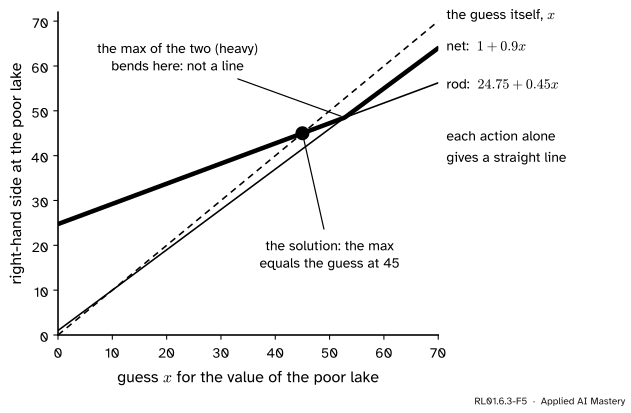
The max makes the equations non-linear. For a fixed policy, the right-hand side is a sum of constants times values: a linear expression, which led to one linear system. A maximum of several linear expressions is not linear.
RL01.6.3-F5
The right-hand side at the poor lake, as a function of a guess for \(v_*(\text{poor})\), with \(v_*(\text{rich})\) held at 55. Each action gives a straight line. Their maximum has a kink. The equation is solved where the heavy line meets the dashed line.
Because of the kink, the optimality equations cannot be solved as one matrix equation. For a tiny problem we can try every policy, as the worked example does, but \(n\) states and \(k\) actions give \(k^n\) deterministic policies. The next lesson shows that, for \(\gamma < 1\), the equations have exactly one solution, and that repetition always finds it.
Worked example
Find the optimal policy of the lake, and verify it. As before, \(\gamma = 0.9\), and \(x\) and \(y\) stand for the values of the rich and the poor lake under the policy in hand.
Evaluate each deterministic policy. Each needs one Bellman equation per state.
Rod in both states.\(x = 2 + 0.9x\) gives \(x = 20\). Then \(y = 0 + 0.9\,(0.5x + 0.5y) = 9 + 0.45y\) gives \(y = 9 / 0.55 \approx 16.36\).
Rod if rich, net if poor. Again \(x = 20\). And \(y = 1 + 0.9y\) gives \(y = 10\).
Net if rich, rod if poor.\(x = 10 + 0.9\,(0.5x + 0.5y)\) and \(y = 0 + 0.9\,(0.5x + 0.5y)\). Subtracting, \(x - y = 10\). Then \(y = 0.45\,(2y + 10) = 0.9y + 4.5\) gives \(y = 45\), and \(x = 55\).
Net in both states.\(y = 1 + 0.9y\) gives \(y = 10\). Then \(x = 10 + 0.9\,(0.5x + 5) = 14.5 + 0.45x\) gives \(x = 14.5 / 0.55 \approx 26.36\).
Policy
Value of rich
Value of poor
rod in both states
20
16.36
rod if rich, net if poor
20
10
net if rich, rod if poor
55
45
net in both states
26.36
10
Pick the best. The third row is the largest in both columns. Some optimal policy is always deterministic (take one maximising action per state), so this row is optimal among all policies: \(v_*(\text{rich}) = 55\) and \(v_*(\text{poor}) = 45\).
Verify with the optimality equation. Forget where the numbers came from and test them.
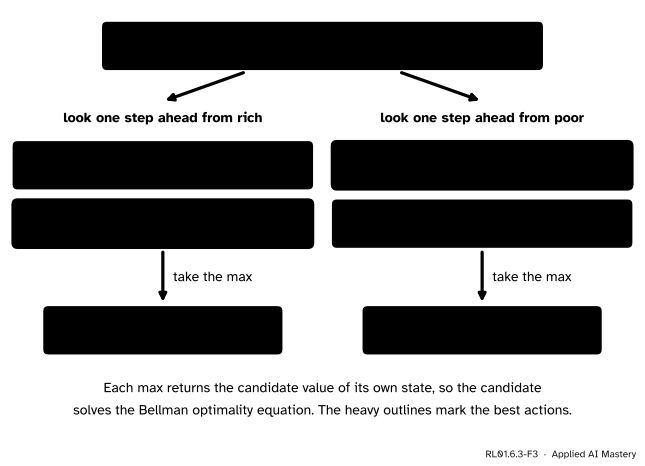
RL01.6.3-F3
Checking the candidates 55 and 45. In each state the larger look-ahead returns that state’s candidate value, as the optimality equation demands.
Here 50 is the average of 55 and 45. The larger look-ahead is 55 at the rich lake and 45 at the poor lake: each state’s candidate value, so both pass. By Link 1 the four numbers are the optimal action values \(q_*(s, a)\), and the greedy policy takes the larger in each state: net when rich, rod when poor.
Code
The search over policies, from scratch, with the model and the solver of the last lesson.
import itertoolsimport numpy as npGAMMA =0.9STATES = ["rich", "poor"]ACTIONS = ["rod", "net"]p = { # p[(state, action)] lists the outcomes as (probability, next state, reward) ("rich", "rod"): [(1.0, "rich", 2)], ("rich", "net"): [(0.5, "rich", 10), (0.5, "poor", 10)], ("poor", "rod"): [(0.5, "rich", 0), (0.5, "poor", 0)], ("poor", "net"): [(1.0, "poor", 1)],}def evaluate(plan):"""Values of a deterministic policy {state: action}: solve (I - gamma P) v = r.""" P, r = np.zeros((2, 2)), np.zeros(2)for i, s inenumerate(STATES):for prob, s2, reward in p[(s, plan[s])]: P[i, STATES.index(s2)] += prob r[i] += prob * rewardreturn np.linalg.solve(np.eye(2) - GAMMA * P, r)plans = [dict(zip(STATES, choice)) for choice in itertools.product(ACTIONS, repeat=2)]values = [evaluate(plan) for plan in plans]print("rich/poor v(rich) v(poor)")for plan, v inzip(plans, values):print(f"{plan['rich']} / {plan['poor']}{v[0]:8.2f}{v[1]:8.2f}")best =max(range(4), key=lambda i: values[i].sum())v_star = {s: float(round(x, 9)) for s, x inzip(STATES, values[best])}print("best plan:", plans[best])print("v* =", v_star)
rich/poor   v(rich)  v(poor)
rod / rod     20.00    16.36
rod / net     20.00    10.00
net / rod     55.00    45.00
net / net     26.36    10.00
best plan: {'rich': 'net', 'poor': 'rod'}
v* = {'rich': 55.0, 'poor': 45.0}
The best plan wins in each state separately. Now verify the optimality equation, and read the greedy policy off the optimal action values.
def look_ahead(v, s, a):"""One-step look-ahead: sum of p * (r + gamma * v(s'))."""returnsum(prob * (r + GAMMA * v[s2]) for prob, s2, r in p[(s, a)])q_star = {(s, a): look_ahead(v_star, s, a) for s in STATES for a in ACTIONS}for s in STATES: row = {a: round(q_star[(s, a)], 2) for a in ACTIONS} greedy =max(ACTIONS, key=lambda a: q_star[(s, a)])print(f"{s}: q* = {row}")print(f" max = {max(row.values())}, greedy action: {greedy}")
rich: q* = {'rod': 51.5, 'net': 55.0}
      max = 55.0, greedy action: net
poor: q* = {'rod': 45.0, 'net': 41.5}
      max = 45.0, greedy action: rod
No library call replaces this search, and it does not scale: a gridworld with 9 open cells and four moves has \(4^9 = 262{,}144\) plans. Modules RL01.7 and RL01.8 build the methods used instead.
Explore
This module’s interactive, the Bellman backup gridworld, lives in lesson RL01.6.4. Switch it between “random policy” and “optimal” to compare the average with the maximum on the same grid.
Pitfalls
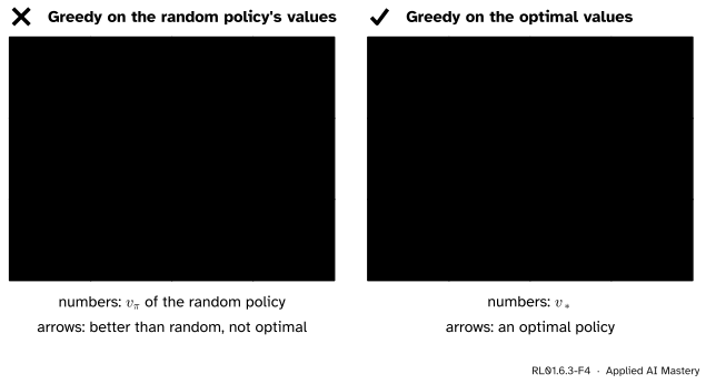
RL01.6.3-F4
Wrong beside right, in the gridworld of this module’s interactive (rules in lesson RL01.6.4; here slip 0.2, reward per step \(-0.04\) and \(\gamma = 0.9\)). The arrows on the left are greedy on the uniform random policy’s values. They differ from the optimal arrows in the two outlined cells.
“Acting greedily on \(v_\pi\) gives the optimal policy.”
It gives a policy that is at least as good as\(\pi\) in every state, and strictly better somewhere unless \(\pi\) was already optimal: the policy improvement theorem (Sutton and Barto, Section 4.2). It need not be optimal. In the figure, the left-hand policy is worth 0.23 in the third cell of the bottom row, where the optimal policy is worth 0.43. Only greed on \(v_*\) is guaranteed optimal. At the lake, greed on the coin-toss values happens to be optimal at once. The gridworld shows this is luck.
“The optimality equation averages over the actions, like the expectation equation.”
Averaging describes a policy that picks actions by chance. An even average at the lake gives back the coin-toss values, 37.5 and 27.5, not 55 and 45. The optimal agent never mixes in a worse action, so its equation takes the maximum.
“Greedy means grabbing the biggest reward now.”
Greedy with respect to \(v_*\) compares reward plus discounted next value, not reward alone. At the poor lake the net wins on reward, 1 against 0, and loses on look-ahead, 41.5 against 45. Comparing rewards alone is the case \(\gamma = 0\): an agent that cannot see past today. This is why reinforcement learning systems learn value functions: a good one turns a hard long-term choice into an easy one-step comparison.
Check yourself
Recall
1. What does it mean for a policy to be optimal?
Show answer
Its value is at least as large as the value of every other policy, in every state.
2. State the Bellman optimality equation for \(v_*\).
Show answer
\(v_*(s) = \max_a \sum_{s', r} p(s', r \mid s, a)\,[\,r + \gamma\, v_*(s')\,]\), for every state \(s\).
3. What is the one difference between the backup diagram for \(v_\pi\) and the one for \(v_*\)?
Show answer
At the top, the average over actions weighted by \(\pi(a \mid s)\) is replaced by a maximum over actions, drawn as an arc.
4. How does an agent choose an action if it knows \(q_*\)? And if it knows only \(v_*\)?
Show answer
With \(q_*\) it picks the action with the largest \(q_*(s, a)\). With \(v_*\) it must look one step ahead with the dynamics \(p\) and take the action with the largest look-ahead.
5. Why can the optimal values not be found by one linear solve?
Show answer
Because of the maximum. A maximum of linear expressions is not linear, so the optimality equations are not a linear system.
Exercises
1.★ A two-action problem has \(q_*(s_1, a_1) = 4\), \(q_*(s_1, a_2) = 7\), \(q_*(s_2, a_1) = 3\) and \(q_*(s_2, a_2) = 1\). Give \(v_*\) and an optimal policy.
Show solution
\(v_*(s) = \max_a q_*(s, a)\), so \(v_*(s_1) = 7\) and \(v_*(s_2) = 3\). An optimal policy takes the maximising action in each state: \(a_2\) in \(s_1\) and \(a_1\) in \(s_2\).
2.★★ Suppose the net at a poor lake caught 6 fish, not 1, with everything else unchanged. Show that 55 and 45 no longer satisfy the optimality equation. Then find the new optimal values by testing the plan “net in both states”.
Show solution
At the poor lake the look-aheads with the old values are \(0 + 0.9 \times 50 = 45\) for the rod and \(6 + 0.9 \times 45 = 46.5\) for the net. The maximum is 46.5, not 45, so the equation fails there.
Evaluate “net in both states”: \(y = 6 + 0.9y\) gives \(y = 60\), and \(x = 10 + 0.9\,(0.5x + 30) = 37 + 0.45x\) gives \(x = 37 / 0.55 \approx 67.27\). Test them. Rich: rod \(2 + 0.9 \times 67.27 = 62.55\), net \(67.27\). Poor: rod \(0.9 \times 63.64 = 57.27\), net \(6 + 0.9 \times 60 = 60\). Each maximum returns its state’s value. The optimality equation has only one solution (next lesson), so \(v_* \approx (67.27,\ 60)\) and the net is now optimal everywhere.
3.★★★ Go back to the original lake, and let the discount rate \(\gamma\) vary. For which values of \(\gamma\) is “net when rich, rod when poor” an optimal policy?
Show solution
Let \(x\) and \(y\) be the values of this plan. Its Bellman equations are \(x = 10 + \tfrac{\gamma}{2}(x + y)\) and \(y = \tfrac{\gamma}{2}(x + y)\). Subtracting gives \(x - y = 10\). Then \(y = \tfrac{\gamma}{2}(2y + 10) = \gamma\,(y + 5)\), so \(y = 5\gamma / (1 - \gamma)\) and \(x = y + 10\).
The plan is optimal exactly when these values satisfy the optimality equation: in each state its own action must be at least as good as the other.
Poor:\(y \ge 1 + \gamma y\), that is \(y\,(1 - \gamma) \ge 1\), that is \(5\gamma \ge 1\), so \(\gamma \ge 0.2\).
Rich:\(x \ge 2 + \gamma x\), that is \(x\,(1 - \gamma) \ge 2\). Now \(x\,(1 - \gamma) = (y + 10)(1 - \gamma) = 5\gamma + 10 - 10\gamma = 10 - 5\gamma \ge 5\), so this always holds.
The plan is optimal for \(0.2 \le \gamma < 1\). Below 0.2 the future counts for too little: one fish from the net beats the chance of a recovered lake.
Summary card
The best value of a state is the best one-step look-ahead: reward plus discounted best value of what follows.
RL01.6.3-F1
Look ahead, keep the best.
Optimal values.\(v_*(s) = \max_\pi v_\pi(s)\) and \(q_*(s, a) = \max_\pi q_\pi(s, a)\).
For action values.\(q_*(s, a) = \sum_{s', r} p(s', r \mid s, a)\,[\,r + \gamma \max_{a'} q_*(s', a')\,]\).
Links.\(v_*(s) = \max_a q_*(s, a)\). A policy that is greedy with respect to \(v_*\) or \(q_*\) is optimal.
At the lake.\(v_* = (55,\ 45)\): net when the lake is rich, rod when it is poor.
Sources and next steps
Sources. Each was opened and checked against this lesson on 12 November 2026.
Richard S. Sutton and Andrew G. Barto, Reinforcement Learning: An Introduction, 2nd edition, MIT Press, 2018. Section 3.6 defines \(v_*\) and \(q_*\) in equations (3.15) and (3.16), relates them in (3.17), and gives the Bellman optimality equations as (3.19) for \(v_*\) and (3.20) for \(q_*\), with the backup diagrams of Figure 3.4. It states that an optimal policy always exists, that any policy greedy with respect to \(v_*\) is optimal, and that \(q_*\) makes the one-step search unnecessary. Section 4.2 gives the policy improvement theorem, (4.7) and (4.8). Section 5.2 explains that without a model, state values alone cannot give a policy, and Section 6.5 that Q-learning approximates \(q_*\) directly.
David Silver, Reinforcement Learning, lecture course (Advanced Topics 2015), Lecture 2: Markov Decision Processes. The slide “Solving the Bellman Optimality Equation” notes that the equation is non-linear, with no closed form in general.
Csaba Szepesvári, Algorithms for Reinforcement Learning, the author’s draft. Section 2.3 gives the Bellman optimality equation as (12). Appendix A.2 proves that a policy greedy with respect to its solution is optimal (Theorem 2), and the policy improvement theorem (Theorem 3).
Joshua Achiam, Part 1: Key Concepts in RL, OpenAI Spinning Up. The section “Bellman Equations” names the max over actions as the crucial difference between the two kinds of equation.
Next.RL01.6.4 Bellman backups as operators treats the right-hand sides of both equations as machines that act on any table of values, and proves that repeating them converges when \(\gamma < 1\).