For a fixed policy, the value of every state is tied to the values of the states that can follow it. Derive that tie, the Bellman expectation equation, line by line from the definition of value, read it off a backup diagram, and solve it as a small system of linear equations by hand and with NumPy.
Derive the Bellman expectation equation for state values from the definition of value, naming the rule of probability used at each step.
Read a backup diagram and write the equation it stands for.
Convert between state values and action values of a policy in both directions.
Evaluate a fixed policy on a small Markov decision process by solving its Bellman equations as a linear system, by hand and with NumPy.
Explain why the linear system has exactly one solution when the discount rate is below 1.
In review. The maths and code on this page are checked by automated tests on every change, but an independent reader has not signed it off yet. Spot a mistake or a confusing step? Tell us.
The question
A fisher decides each morning by tossing a coin: rod or net. How many fish is a rich lake worth to this fisher in the long run? The value of the rich lake depends on the value of the poor lake, because the net can empty the lake. The value of the poor lake depends on the value of the rich lake, because the lake can recover. How do you find two numbers that are each defined by the other?
From the last lesson
1. Write the return \(G_t\) in terms of the next reward and the next return.
Show answer
\(G_t = R_{t+1} + \gamma\, G_{t+1}\).
2. What is the difference between a return and a value?
Show answer
A return is the discounted sum of rewards along one run, so it is random. The value of a state is the expected return from that state under a policy: one number per state.
Intuition
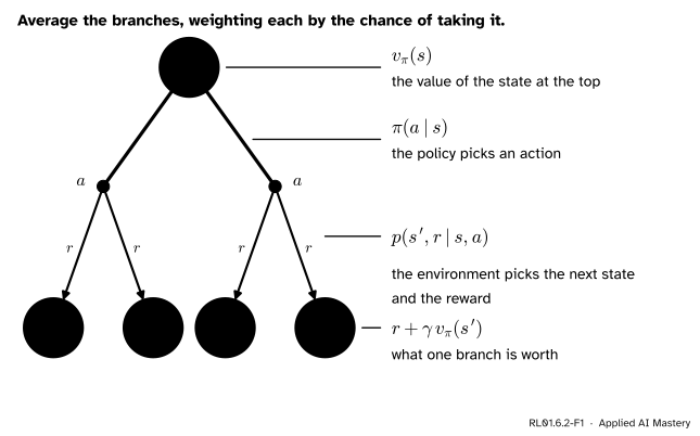
Stand in a state \(s\) and follow a policy \(\pi\) for one step. Two things happen, in this order.
The policy picks an action. It picks \(a\) with probability \(\pi(a \mid s)\).
The environment picks the outcome. It moves to state \(s'\) and pays reward \(r\) with probability \(p(s', r \mid s, a)\).
After that step the agent holds a reward \(r\) and stands in \(s'\), from where the rest of the future is worth \(v_\pi(s')\) on average. So this one branch is worth \(r + \gamma\, v_\pi(s')\). The value of \(s\) is the average of that quantity over all the branches.
RL01.6.2-F1
The backup diagram for the value of a state. An open circle is a state and a solid dot is an action. The value at the top is the average of what the branches are worth. The weight of a branch is the policy’s probability of its action times the environment’s probability of its outcome.
The picture is called a backup diagram because information flows back up it: from the values at the bottom to the value at the top.
There is a catch. The states at the bottom are ordinary states, and their values are as unknown as the one at the top. So the diagram does not hand us \(v_\pi(s)\). It gives one equation that links \(v_\pi(s)\) to the other values. One diagram per state gives one equation per state, and solving them together gives the values.
Build it up
Use the lake of the last lesson, with \(\gamma = 0.9\), and the coin-toss policy: in either state, rod with probability 0.5 and net with probability 0.5.
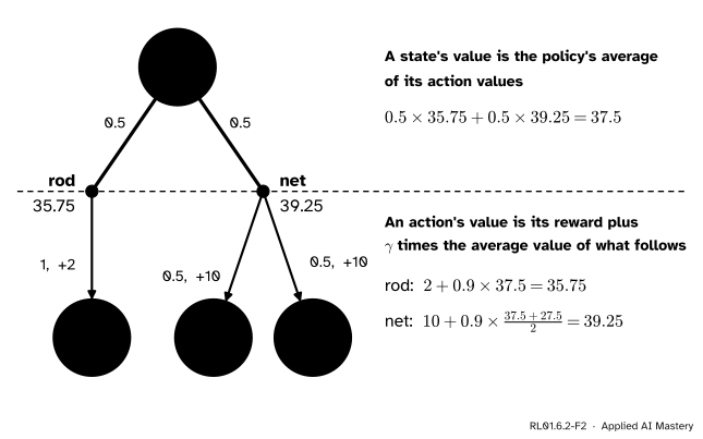
Step 1. Look ahead from an action. Suppose the values at the bottom were known. Looking ahead from a dot then gives the value of that action: its reward plus \(\gamma\) times the average value of the states it leads to. This is the action value\(q_\pi(s, a)\).
Step 2. Average over the actions. The state at the top takes each action with the policy’s probability. So its value is the policy’s average of the action values.
RL01.6.2-F2
Both steps at the rich lake, using the values that the worked example will find: 37.5 for rich and 27.5 for poor. The bottom half turns state values into action values. The top half turns action values back into a state value.
Step 3. Join the two steps. Put Step 1 inside Step 2. The action values drop out, and what is left links the value at the top directly to the values at the bottom. That link is the Bellman expectation equation.
Step 4. Notice the loop. In the figure, rich appears at the top and again at the bottom: 37.5 is used to compute itself. This is no mistake. 37.5 and 27.5 are the pair of numbers that make every such diagram balance at once.
The formal statement
NoteDefinitions: the two value functions of a policy
The state-value function is the expected return from a state, and the action-value function is the expected return after a given first action, when \(\pi\) is followed afterwards:
The colours match the backup diagram: the policy, the environment, the values and the discount. The sum over \(s', r\) runs over every pair of next state and reward.
Derivation. One rule of probability does most of the work. If a list of cases covers every possibility and no two cases can happen together, then an average is the sum over the cases of (probability of the case) × (average within the case). This is the law of total expectation:
Here a case is a triple \((a, s', r)\): the event that \(A_t = a\), \(S_{t+1} = s'\) and \(R_{t+1} = r\). Given \(S_t = s\), the policy first picks \(a\) and then the environment picks \((s', r)\), so by the product rule
The second term. Split it into the same cases. Write \(\E_\pi[\,G_{t+1} \mid s, a, s', r\,]\) for the average of \(G_{t+1}\) given \(S_t = s\) and the case \((a, s', r)\):
The inner average simplifies because of the Markov property. \(G_{t+1}\) is made of the rewards \(R_{t+2}, R_{t+3}, \dots\) All of them are produced from \(S_{t+1}\) onwards, by a policy that looks only at the current state and by dynamics \(p\) that look only at the current state and action. Once we know \(S_{t+1} = s'\), the earlier facts \(S_t = s\), \(A_t = a\) and \(R_{t+1} = r\) tell us nothing more about those rewards. So
The last equality is the definition of \(v_\pi\) again, used at time \(t + 1\). It applies at any time step, because neither the policy nor the dynamics change with time.
Put the terms back. Both terms are sums with the same weights, so they combine:
\[
\begin{aligned}
& v_\pi(s) \\
&\; = \sum_{a} \pi(a \mid s) \sum_{s', r} p(s', r \mid s, a)\, r \\
&\;\quad + \gamma \sum_{a} \pi(a \mid s) \sum_{s', r} p(s', r \mid s, a) \\
&\;\qquad\quad \times\; v_\pi(s') \\
&\; = \sum_{a} \pi(a \mid s) \sum_{s', r} p(s', r \mid s, a) \\
&\;\qquad \times\; \big[ r + \gamma v_\pi(s') \big] .
\end{aligned}
\]
That is the equation in the box, (3.14) in Sutton and Barto.
Action values. Repeat the derivation with the first action fixed at \(a\). Nothing is averaged over the policy at the first step, so the outer sum disappears:
\[
\begin{aligned}
q_\pi(s, a) = {} & \sum_{s', r} p(s', r \mid s, a) \\
& \times \big[ r + \gamma\, v_\pi(s') \big] .
\end{aligned}
\]
Call this relation q from v. In the other direction, split \(\E_\pi[G_t \mid S_t = s]\) into cases by the first action alone. That gives v from q:
These are Steps 1 and 2 of the last section. Putting the first into the second gives the Bellman equation for \(v_\pi\) again. The second into the first gives the one for \(q_\pi\):
\[
\begin{aligned}
& q_\pi(s, a) = \sum_{s', r} p(s', r \mid s, a) \\
&\quad \times \Big[ r + \gamma \sum_{a'} \pi(a' \mid s')\, q_\pi(s', a') \Big] .
\end{aligned}
\]
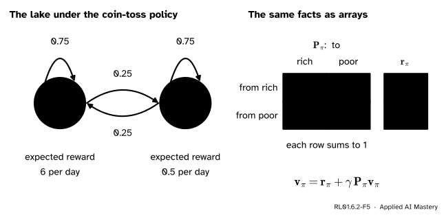
Matrix form. For a fixed policy only two things matter about a step: the reward it pays on average, and where it leads. Collect them as
\(r_\pi(s)\) is the expected reward of one step from \(s\), and \(P_\pi(s, s')\) is the probability that the step ends in \(s'\).
RL01.6.2-F5
Once the policy is fixed, the actions can be averaged away. The lake becomes a chain that moves between two states and pays an expected reward in each. The matrix \(\mat{P}_\pi\) and the vector \(\vect{r}_\pi\) hold the same information.
With these, the Bellman equation reads \(v_\pi(s) = r_\pi(s) + \gamma \sum_{s'} P_\pi(s, s')\, v_\pi(s')\). Stack the values into a vector \(\vect{v}_\pi\), the rewards into \(\vect{r}_\pi\) and the probabilities into a matrix \(\mat{P}_\pi\) with one row per starting state. Then move the unknowns to the left and multiply by the inverse:
The Bellman expectation equation is a system of linear equations: as many equations as states, and as many unknowns.
Go deeper: why the inverse exists when the discount rate is below 1
A square matrix has an inverse exactly when the only vector it sends to zero is the zero vector. So suppose \((\mat{I} - \gamma \mat{P}_\pi)\,\vect{x} = \vect{0}\), which says \(\vect{x} = \gamma\, \mat{P}_\pi \vect{x}\). We show that \(\vect{x}\) must be zero.
Let \(m\) be the largest absolute value among the entries of \(\vect{x}\), and let \(i\) be an entry where it is reached, so \(\abs{x_i} = m\). Row \(i\) of the equation says \(x_i = \gamma \sum_j P_\pi(i, j)\, x_j\). Take absolute values. The entries of a row of \(\mat{P}_\pi\) are probabilities: none is negative, and they sum to 1. So
Hence \((1 - \gamma)\, m \le 0\). Since \(\gamma < 1\) and \(m \ge 0\), this forces \(m = 0\): every entry of \(\vect{x}\) is zero. So the matrix is invertible, and the Bellman equation has exactly one solution. As \(v_\pi\) is a solution, by the derivation above, \(v_\pi\) is the solution.
If some states are terminal, leave them out of the vectors. A row of \(\mat{P}_\pi\) may then sum to less than 1, which only helps the inequality.
Worked example
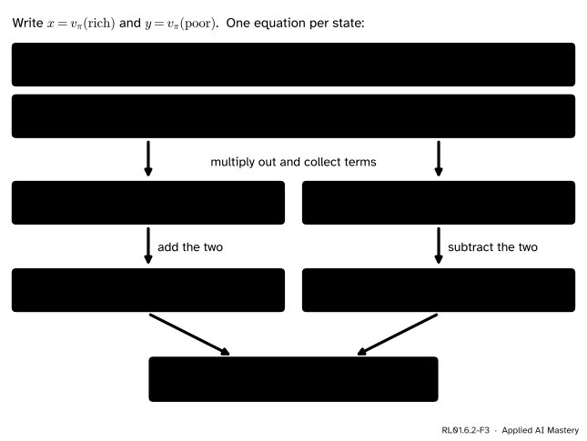
Evaluate the coin-toss policy at the lake. Write \(x = v_\pi(\text{rich})\) and \(y = v_\pi(\text{poor})\), and write the Bellman equation once for each state. The outcomes come from the last lesson’s lake diagram.
At the rich lake, the rod pays 2 and keeps the lake rich. The net pays 10 and leaves the lake rich or poor with probability 0.5 each:
The whole calculation: two equations, simplified and then solved together.
Multiply out. In the first equation, \(0.5 \times 2 + 0.5 \times 10 = 6\), the coefficient of \(x\) is \(0.5 \times 0.9 + 0.5 \times 0.9 \times 0.5 = 0.675\), and the coefficient of \(y\) is \(0.5 \times 0.9 \times 0.5 = 0.225\). The second equation works the same way:
\[
\begin{aligned}
x &= 6 + 0.675x + 0.225y, \\
y &= 0.5 + 0.225x + 0.675y .
\end{aligned}
\]
Add the two equations: \(x + y = 6.5 + 0.9\,(x + y)\), so \(0.1\,(x + y) = 6.5\) and \(x + y = 65\). Subtract the second from the first: \(x - y = 5.5 + 0.45\,(x - y)\), so \(0.55\,(x - y) = 5.5\) and \(x - y = 10\). Therefore
\[
\begin{aligned}
v_\pi(\text{rich}) &= x = 37.5, \\
v_\pi(\text{poor}) &= y = 27.5 .
\end{aligned}
\]
Check with the action values\(q_\pi(s, a)\). Using q from v:
Here \(32.5 = 0.5 \times 37.5 + 0.5 \times 27.5\) is the average value after an even split. Using v from q: \(0.5 \times 35.75 + 0.5 \times 39.25 = 37.5\) and \(0.5 \times 29.25 + 0.5 \times 25.75 = 27.5\). Both balance.
The same answer from the matrix form. The collected equations give \(\vect{r}_\pi\) and \(\mat{P}_\pi\) directly: \(r_\pi = (6,\ 0.5)\), and, for example, \(P_\pi(\text{rich}, \text{rich}) = 0.5 \times 1 + 0.5 \times 0.5 = 0.75\). So
and solving \((\mat{I} - \gamma \mat{P}_\pi)\,\vect{v}_\pi = \vect{r}_\pi\) is the same pair of equations as before, with the unknowns moved to the left.
Code
First from scratch. The lake is a dictionary of outcomes, and one function computes the right-hand side of the Bellman equation for any table of values. Feeding it the hand-solved values should return them unchanged.
GAMMA =0.9STATES = ["rich", "poor"]ACTIONS = ["rod", "net"]# p[(state, action)] lists the outcomes as (probability, next state, reward).p = { ("rich", "rod"): [(1.0, "rich", 2)], ("rich", "net"): [(0.5, "rich", 10), (0.5, "poor", 10)], ("poor", "rod"): [(0.5, "rich", 0), (0.5, "poor", 0)], ("poor", "net"): [(1.0, "poor", 1)],}coin_toss = {s: {"rod": 0.5, "net": 0.5} for s in STATES}def q_from_v(v, s, a):"""Look ahead from an action: sum of p * (r + gamma * v(s'))."""returnsum(prob * (r + GAMMA * v[s2]) for prob, s2, r in p[(s, a)])def bellman_rhs(v, pi):"""The right-hand side of the Bellman expectation equation, for every state."""return {s: sum(pi[s][a] * q_from_v(v, s, a) for a in ACTIONS) for s in STATES}v_hand = {"rich": 37.5, "poor": 27.5}print("right-hand side:", bellman_rhs(v_hand, coin_toss))for s in STATES:for a in ACTIONS:print(f"q({s}, {a}) = {q_from_v(v_hand, s, a):.2f}")
The right-hand side returns 37.5 and 27.5, so the hand-solved values satisfy the equation. Now the library route: build \(\mat{P}_\pi\) and \(\vect{r}_\pi\), and let NumPy solve the linear system.
import numpy as npdef policy_matrices(pi):"""P_pi[i, j] = probability of moving from state i to state j. r_pi[i] = expected reward from i.""" n =len(STATES) P, r = np.zeros((n, n)), np.zeros(n)for i, s inenumerate(STATES):for a in ACTIONS:for prob, s2, reward in p[(s, a)]: P[i, STATES.index(s2)] += pi[s][a] * prob r[i] += pi[s][a] * prob * rewardreturn P, rP_pi, r_pi = policy_matrices(coin_toss)v_pi = np.linalg.solve(np.eye(2) - GAMMA * P_pi, r_pi)print("P_pi =", P_pi.tolist())print("r_pi =", r_pi.tolist())print("v_pi =", np.round(v_pi, 6).tolist())
np.linalg.solve is preferred to forming the inverse: a direct solve can be faster and more numerically stable. Its cost still grows with the cube of the number of states, so it suits small problems. Lesson RL01.6.4 gives a route that scales better.
Explore
This module’s interactive, the Bellman backup gridworld, lives in lesson RL01.6.4. Its “random policy” mode applies the right-hand side of this lesson’s equation to every cell of a grid, again and again.
Pitfalls
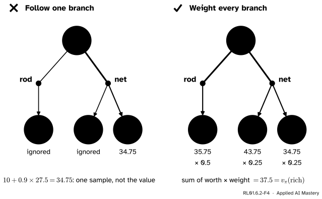
RL01.6.2-F4
Wrong beside right. One branch is one sample of what might happen. The value averages every branch, weighted by policy probability times environment probability.
“To get the value, follow what happens next: reward plus \(\gamma\) times the value of the next state.”
That is one branch. The Bellman equation averages over all actions and all outcomes. One observed step gives \(r + \gamma\, v_\pi(s')\) for a single triple \((a, s', r)\), which equals \(v_\pi(s)\) only on average. Temporal-difference learning (RL02.2) does use single steps, and must average many of them for this reason.
“The Bellman equation is a formula: plug in numbers on the right and read off the value.”
The unknown values appear on both sides. With zeros on the right, the lake’s equations return 6 and 0.5, not 37.5 and 27.5. The equation is a condition that the true values satisfy, so it has to be solved. Lesson RL01.6.4 shows that repeated plugging-in does get there.
“A state has a value.”
A state has a value under a policy. The rich lake is worth 37.5 to the coin-tossing fisher and 55 to the fisher of the last lesson (net when rich, rod when poor). Always say which policy a value belongs to: that is what the subscript in \(v_\pi\) is for.
Check yourself
Recall
1. In a backup diagram, what do the open circles and the solid dots stand for?
Show answer
An open circle is a state. A solid dot is an action taken in a state (a state-action pair).
2. State the Bellman expectation equation for \(v_\pi\).
Show answer
\(v_\pi(s) = \sum_a \pi(a \mid s) \sum_{s', r} p(s', r \mid s, a)\,[\,r + \gamma\, v_\pi(s')\,]\), for every state \(s\).
3. How do you get \(v_\pi(s)\) from the action values \(q_\pi(s, a)\)?
Show answer
Average them with the policy’s probabilities: \(v_\pi(s) = \sum_a \pi(a \mid s)\, q_\pi(s, a)\).
4. Which property lets us replace the expected next return, given the whole past, by \(v_\pi(s')\)?
Show answer
The Markov property: once the next state \(s'\) is known, the earlier state, action and reward tell us nothing more about the rewards that follow.
5. Write the Bellman expectation equation in matrix form, and its solution.
1.★ A fisher uses the net with probability 0.2 and the rod with probability 0.8 in both states. Find \(\vect{r}_\pi\) and \(\mat{P}_\pi\) for the lake.
Show solution
Expected rewards: \(r_\pi(\text{rich}) = 0.8 \times 2 + 0.2 \times 10 = 3.6\) and \(r_\pi(\text{poor}) = 0.8 \times 0 + 0.2 \times 1 = 0.2\). From rich, the lake stays rich with probability \(0.8 \times 1 + 0.2 \times 0.5 = 0.9\). From poor, it becomes rich with probability \(0.8 \times 0.5 + 0.2 \times 0 = 0.4\). So
2.★★ Evaluate the policy “always use the rod” at the lake by writing and solving its two Bellman equations.
Show solution
Let \(x\) and \(y\) be the values of rich and poor. At the rich lake the rod pays 2 and the lake stays rich: \(x = 2 + 0.9x\), so \(x = 20\). At the poor lake the rod pays 0 and the lake is rich or poor with probability 0.5 each: \(y = 0 + 0.9\,(0.5x + 0.5y) = 9 + 0.45y\), so \(0.55y = 9\) and \(y = 9 / 0.55 \approx 16.36\). Both are below the coin-toss values.
3.★★★ Use the matrix form to show that adding the same constant \(c\) to every reward raises the value of every state by \(c / (1 - \gamma)\), whatever the policy. Assume \(\gamma < 1\) and no terminal states.
Show solution
Let \(\vect{1}\) be the vector of ones. Adding \(c\) to every reward changes \(\vect{r}_\pi\) to \(\vect{r}_\pi + c\,\vect{1}\), because the probabilities in each expected reward sum to 1. \(\mat{P}_\pi\) does not change. Try \(\vect{v}_\pi + k\,\vect{1}\) as the new solution. Every row of \(\mat{P}_\pi\) sums to 1, so \(\mat{P}_\pi \vect{1} = \vect{1}\), and
This equals \(\vect{r}_\pi + c\,\vect{1}\) exactly when \(k = c / (1 - \gamma)\). The solution is unique, so the new values are \(\vect{v}_\pi + \tfrac{c}{1 - \gamma}\vect{1}\). With \(\gamma = 0.9\), one extra fish per day is worth 10 in every state.
Summary card
The value of a state is the weighted average of reward plus discounted next value, over every branch of one step.
At the lake, tossing a coin.\(v_\pi(\text{rich}) = 37.5\) and \(v_\pi(\text{poor}) = 27.5\).
Sources and next steps
Sources. Each was opened and checked against this lesson on 12 November 2026.
Richard S. Sutton and Andrew G. Barto, Reinforcement Learning: An Introduction, 2nd edition, MIT Press, 2018. Section 3.5 defines \(v_\pi\) and \(q_\pi\) in equations (3.12) and (3.13), derives the Bellman equation for \(v_\pi\) as (3.14) and introduces the backup diagram, with open circles for states and solid circles for state-action pairs. Exercises 3.12 and 3.13 ask for the two relations between \(v_\pi\) and \(q_\pi\). Section 4.1 notes that it is a system of linear equations, one per state. Section 6.1: a TD target samples this expectation.
David Silver, Reinforcement Learning, lecture course (Advanced Topics 2015), Lecture 2: Markov Decision Processes. The slide “Bellman Expectation Equation (Matrix Form)” gives \(v_\pi = \mathcal{R}^\pi + \gamma \mathcal{P}^\pi v_\pi\) and the direct solution \(v_\pi = (I - \gamma \mathcal{P}^\pi)^{-1} \mathcal{R}^\pi\). The slide “Solving the Bellman Equation” gives the cost of a direct solution as \(O(n^3)\).
Csaba Szepesvári, Algorithms for Reinforcement Learning, the author’s draft. Section 2.3 writes the Bellman equation of a policy in the compact form \(r^\pi + \gamma P^\pi V^\pi = V^\pi\), equation (11), and states that it has a unique solution when \(0 < \gamma < 1\).
SciPy, Linear Algebra tutorial, “Solving a linear system”: a solve “can be faster and more numerically stable” than the inverse. NumPy’s solve calls LAPACK’s _gesv.