The discounted return hides a copy of itself: the return from now is the first reward plus the discount times the return from the next step. Derive that recursion, use it to work backwards along a chain of rewards, and meet the one-step look-ahead that every Bellman equation is built on.
Derive the recursion that writes the return as the first reward plus the discount times the next return, from the definition of the discounted return.
Compute every return along a finite sequence of rewards by working backwards from the end.
Explain the difference between a return, which belongs to one run, and a value, which is an average over runs.
Check a table of state values with a one-step look-ahead: reward now plus the discounted average value of the next state.
In review. The maths and code on this page are checked by automated tests on every change, but an independent reader has not signed it off yet. Spot a mistake or a confusing step? Tell us.
The question
A fisher can take ten fish from the lake today with a net, or two with a rod. The big catch may leave the lake poor for days. The worth of today’s choice depends on rewards that keep arriving with no end. How can anyone add up an endless future, and why is it enough to look just one step ahead?
Intuition
Module RL01.5 defined the return: the sum of all rewards from now on, where a reward that arrives \(k\) steps later is first multiplied by \(\gamma^k\). The number \(\gamma\) is the discount rate. This module uses \(\gamma = 0.9\) throughout.
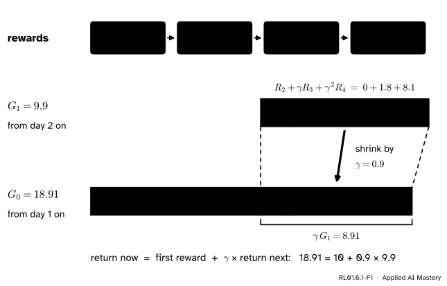
Take four days at the lake with catches of 10, 0, 2 and 10 fish. Seen from day 1, the return is
Now stand on day 2 and ask the same question. Three rewards are left, and the return is \(0 + 0.9 \times 2 + 0.9^2 \times 10 = 9.9\). Put the two sums side by side and something useful appears.
RL01.6.1-F1
The return from day 1, \(G_0\), is the first reward followed by a copy of the next return, \(G_1\), shrunk by the discount. Every later reward is one step further away when seen from day 1, so each picks up one more factor of \(\gamma\).
Every reward after the first is one day further off when you stand one day earlier. So each of them is multiplied by one more \(\gamma\). The whole tail of the day-1 sum is therefore the day-2 sum times \(\gamma\):
\[
18.91 \;=\; 10 \;+\; 0.9 \times 9.9 .
\]
In words: return now = first reward + discount × return next. That one line is the seed of every Bellman equation in this module, and of most learning rules in reinforcement learning.
Build it up
Step 1. Name the parts. Following Sutton and Barto, \(S_t\) is the state at time \(t\), \(A_t\) is the action taken there, and \(R_{t+1}\) is the reward that follows. The return from time \(t\) is called \(G_t\).
Step 2. Split off the first reward.\(G_t\) starts with \(R_{t+1}\), which has no discount at all.
Step 3. Pull one \(\gamma\) out of the rest. Every later term has at least one factor of \(\gamma\). Take one out, and what stays in the bracket is the same kind of sum, started one step later. That sum is \(G_{t+1}\).
Step 4. Use it backwards. If a run of rewards ends, the return after the last reward is zero. From there the rule fills in the returns one at a time, from the end towards the start. The worked example does this for the four days above.
Step 5. Let the future be random. At a real lake, tomorrow is uncertain. Here is the lake that this module uses as its running example.
RL01.6.1-F2
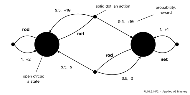
The lake as a Markov decision process. It has two states (the lake is rich or poor in fish) and two actions (fish with the rod or with the net). Each arrow that leaves a dot is labelled probability, reward. The net pays more today but can empty the lake. The rod at a poor lake catches nothing, and gives the lake an even chance to recover.
Read one branch aloud to check the picture: “The lake is rich and the fisher uses the net. The catch is 10. With probability 0.5 the lake is still rich tomorrow, and with probability 0.5 it is poor.”
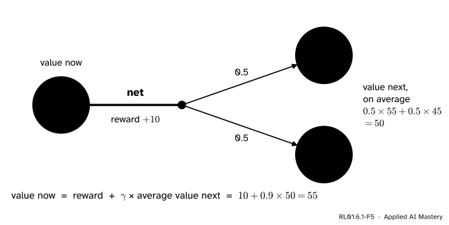
Because tomorrow is random, so is the return. Two runs that start at the same lake with the same plan can collect different totals. The value of a state is the average of those totals: the expected return. Step 3 survives the averaging, and becomes a one-step look-ahead:
RL01.6.1-F5
One step of look-ahead from the rich lake, for a fisher who uses the net when the lake is rich and the rod when it is poor. Under that plan the rich lake is worth 55 and the poor lake 45 (the next two lessons show where these numbers come from). The value now is the reward plus \(\gamma\) times the average value of where the fisher lands.
The formal statement
NoteDefinition: discounted return
For a sequence of rewards \(R_{t+1}, R_{t+2}, R_{t+3}, \dots\) and a discount rate \(0 \le \gamma \le 1\), the return from time \(t\) is
Line 2 takes one common factor \(\gamma\) out of every term after the first. Line 3 recognises the bracket: it is the definition of the return again, with every index moved up by one. The same three lines in summation form, with the substitution \(j = k - 1\) in the last step, read
The final sum is \(G_{t+1}\). For a task that ends at time \(T\), the recursion holds for every \(t < T\), and the convention \(G_T = 0\) makes it true at the last step too: \(G_{T-1} = R_T + \gamma \cdot 0\). This is equation (3.9) of Sutton and Barto.
Go deeper: is it safe to pull a factor out of an endless sum?
Only if the sum settles on a finite number. Suppose every reward lies between \(-R_{\max}\) and \(R_{\max}\), and \(\gamma < 1\). Then the terms of \(G_t\) are no larger in size than those of the geometric series \(R_{\max}(1 + \gamma + \gamma^2 + \cdots) = R_{\max} / (1 - \gamma)\), which is finite. So the series for \(G_t\) converges, and a convergent series can be multiplied or divided by a constant term by term. At the lake no reward is above 10 or below 0, so every return lies between 0 and \(10 / (1 - 0.9) = 100\).
With \(\gamma = 1\) this protection is gone, and an endless run of rewards can add up to infinity. Sutton and Barto (Section 3.4) therefore allow an endless task or \(\gamma = 1\), but not both. Lesson RL01.6.4 shows what goes wrong at the lake.
From returns to values. A policy\(\pi\) is a rule for choosing actions: \(\pi(a \mid s)\) is the probability of action \(a\) in state \(s\). The value of state \(s\) under \(\pi\) is the expected return when the agent starts in \(s\) and follows \(\pi\):
This is the one-step look-ahead of the last figure: value now = expected reward + discount × expected value next. The step from \(G_{t+1}\) to \(v_\pi(S_{t+1})\) was argued in words here. It relies on the Markov property, and the next lesson proves it line by line.
Frontier note: the same line inside deep reinforcement learning
Learning methods rarely know the probabilities of the environment, so they cannot take the average over next states. They use the look-ahead on one observed step instead: after seeing a reward \(r\) and a next state \(s'\), the number \(r + \gamma \times (\text{current estimate at } s')\) serves as a target for the estimate at the state just left. Temporal-difference learning (RL02.2) uses exactly this target. Q-learning (RL02.4) and the deep Q-network (RL03.2) use the same shape with action values: their estimate at \(s'\) is the largest action value there.
Worked example
Part 1: a chain with no randomness. Four days are left in the season. The plan and the luck are fixed, so the rewards are known: \(R_1 = 10\), \(R_2 = 0\), \(R_3 = 2\), \(R_4 = 10\). Find the return from every day, with \(\gamma = 0.9\).
RL01.6.1-F3
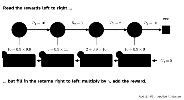
The returns of the chain, filled in from the end. Each green arrow is one use of \(G_t = R_{t+1} + \gamma\, G_{t+1}\).
Start where the answer is known. After the last reward nothing is left, so \(G_4 = 0\). Then step back one day at a time, each time with \(G_t = R_{t+1} + \gamma\, G_{t+1}\):
Check \(G_0\) against the definition: \(10 + 0.9 \times 0 + 0.81 \times 2 + 0.729 \times 10 = 18.91\). The two routes agree. The backward route used four multiplications. The direct route needs a fresh sum, with fresh powers of \(\gamma\), for every starting day.
Nothing in this chain is random, so each state has only one possible return. Its value is that return: the value of \(S_2\) is 11.
Part 2: a look-ahead with randomness. Go back to the lake of the second figure, and to the fisher who uses the net when the lake is rich and the rod when it is poor. Someone claims that under this plan the rich lake is worth 55 and the poor lake 45. Test the claim with one step of look-ahead from each state.
From the rich lake, the net pays 10, and the lake is then rich or poor with probability 0.5 each:
Both checks return the claimed values, so the claim is consistent with itself. A wrong claim fails: try 60 and 45, and the first line gives \(10 + 0.9 \times 52.5 = 57.25\), not 60. The next lesson turns this test into a way of finding the values.
Code
First from scratch. One function follows the recursion from the end of the list. The other follows the definition, so the two can be compared.
def returns_backwards(rewards, gamma):"""The return from every time step, filled in from the end: G_t = R_{t+1} + gamma * G_{t+1}.""" G =0.0# nothing is left after the last reward out = []for r inreversed(rewards): G = r + gamma * G out.append(G)return out[::-1] # back into time orderdef return_direct(rewards, gamma, t=0):"""The definition: the sum of gamma^k * R_{t+k+1} over the rewards that remain."""returnsum(gamma ** k * r for k, r inenumerate(rewards[t:]))rewards = [10, 0, 2, 10] # rewards[t] is R_{t+1}gamma =0.9G = returns_backwards(rewards, gamma)print("backwards", [round(g, 4) for g in G])print("direct ", [round(return_direct(rewards, gamma, t), 4) for t inrange(4)])
backwards [18.91, 9.9, 11.0, 10.0]
direct    [18.91, 9.9, 11.0, 10.0]
Both lines print the values of the figure. The library version treats the recursion as a filter run over the reversed list, which is fast on long arrays. A test on random rewards confirms that all three methods agree.
import numpy as npfrom scipy.signal import lfilterdef returns_filter(rewards, gamma):"""The same recursion, written as a first-order filter over the reversed rewards."""return lfilter([1.0], [1.0, -gamma], np.asarray(rewards, dtype=float)[::-1])[::-1]rng = np.random.default_rng(0)noise = rng.normal(size=500)fast = returns_filter(noise, 0.9)slow = returns_backwards(list(noise), 0.9)print("largest gap:", float(np.max(np.abs(fast - slow))))
largest gap: 0.0
Last, the claim that a value is an average of returns. The cell below plays 20,000 runs of the lake under the plan “net when rich, rod when poor” and averages the returns. Under that plan the lake is rich the next day with probability 0.5, whatever it was today.
def average_return(start_rich, runs=20_000, days=200, gamma=0.9, seed=1): rng = np.random.default_rng(seed) rich = np.full(runs, start_rich) # True where the lake is rich today total = np.zeros(runs)for k inrange(days): reward = np.where(rich, 10.0, 0.0) # net at a rich lake: 10. Rod at a poor lake: 0 total += gamma ** k * reward rich = rng.random(runs) <0.5# rich tomorrow with probability 0.5return total.mean()v_rich, v_poor = average_return(True), average_return(False)print(f"average return, rich lake: {v_rich:.2f}")print(f"average return, poor lake: {v_poor:.2f}")
average return, rich lake: 55.06
average return, poor lake: 45.06
The averages land close to 55 and 45, the values that passed the look-ahead test. Each run stops after 200 days. That is safe, because a reward 200 days away is multiplied by \(0.9^{200}\), which is below one part in a billion.
Explore
This module’s interactive, the Bellman backup gridworld, lives in lesson RL01.6.4. It repeats the one-step look-ahead of this lesson in every cell of a small grid, and shows the numbers in each cell settling down.
Pitfalls
RL01.6.1-F4
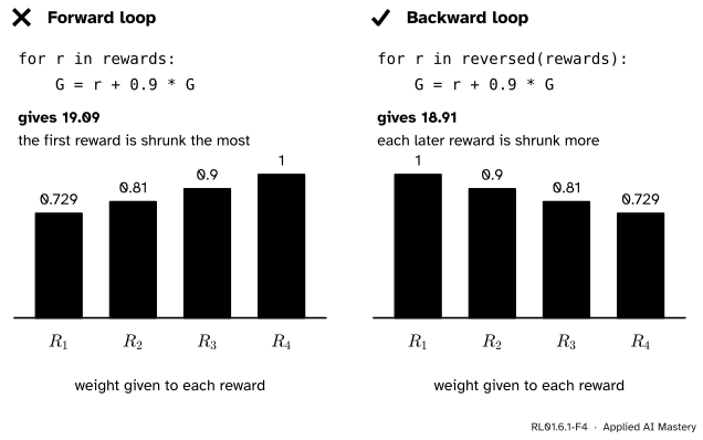
Wrong beside right. The same line of code, run over the rewards in two orders. Run forwards, it discounts the earliest reward the most, which is the opposite of the definition.
“I can add up the return in one pass from the first reward to the last with G = r + gamma * G.”
That update belongs to a backward pass. Run forwards over 10, 0, 2, 10 it gives 19.09 instead of 18.91, because each new step multiplies everything collected so far by \(\gamma\). A correct forward pass needs a separate running power of \(\gamma\): G += discount * r, then discount *= gamma.
“The first reward is discounted too.”
In \(G_t\) the reward \(R_{t+1}\) has weight \(\gamma^0 = 1\). The index looks late, but \(R_{t+1}\) is the immediate reward: it is the result of the action \(A_t\) taken at time \(t\). A formula that starts with \(\gamma R_{t+1}\) shrinks every return by a factor of \(\gamma\).
“The return and the value are the same thing.”
A return belongs to one run, and it changes from run to run when the environment or the policy is random. A value is one fixed number for each state: the average of the returns over all runs. The two agree when nothing is random, as in the chain of Part 1, because every run then collects the same return. Mixing them up matters in machine learning, because an agent only ever sees returns and has to estimate values from them.
Check yourself
Recall
1. Write the return \(G_t\) in terms of the next reward and the next return.
Show answer
\(G_t = R_{t+1} + \gamma\, G_{t+1}\).
2. A task ends at time \(T\). What is \(G_T\), and why?
Show answer
\(G_T = 0\). No rewards are left after the end, and this choice makes the recursion true at the last step: \(G_{T-1} = R_T + \gamma \times 0\).
3. In which direction do you sweep through a list of rewards to compute all the returns with one multiplication per step?
Show answer
Backwards, from the last reward to the first, using \(G = r + \gamma G\) at each step.
4. What is the difference between a return and a value?
Show answer
A return is the discounted sum of rewards along one run, so it is random. The value of a state is the expected return from that state under a policy: one number per state.
5. State the one-step look-ahead for the value of a state in words.
Show answer
Value now equals the expected reward plus the discount times the expected value of the next state.
Exercises
1.★ The rewards of an episode are \(R_1 = 3\), \(R_2 = -1\), \(R_3 = 4\), and \(\gamma = 0.5\). Compute \(G_2\), \(G_1\) and \(G_0\) backwards, and check \(G_0\) with the definition.
2.★★ An agent receives the same reward \(c\) at every step, for ever, with \(\gamma < 1\). Use the recursion, not the formula for a geometric series, to find its return. Then give the return of a fisher who uses the rod at a rich lake every day.
Show solution
Every step looks the same, so the return is the same number \(G\) at every time. The recursion gives \(G = c + \gamma G\), so \(G(1 - \gamma) = c\) and \(G = c / (1 - \gamma)\). The rod at a rich lake pays 2 and leaves the lake rich, so \(c = 2\) and \(G = 2 / (1 - 0.9) = 20\).
3.★★★ A fisher at the lake of this lesson always uses the net. Let \(x\) be the value of the rich lake and \(y\) the value of the poor lake under this plan. Write a one-step look-ahead for each state and solve for \(x\) and \(y\).
Show solution
At a poor lake the net pays 1 and the lake stays poor, so \(y = 1 + 0.9y\), which gives \(y = 1 / 0.1 = 10\). At a rich lake the net pays 10, and the lake is then rich or poor with probability 0.5 each, so \(x = 10 + 0.9\,(0.5x + 0.5y) = 10 + 0.45x + 4.5\). Hence \(0.55x = 14.5\) and \(x = 14.5 / 0.55 \approx 26.36\). Always using the net is worth far less than the 55 and 45 of the plan in the worked example.
Summary card
The return from now is the first reward plus a discounted copy of the return from the next step.
Sources. Each was opened and checked against this lesson on 12 November 2026.
Richard S. Sutton and Andrew G. Barto, Reinforcement Learning: An Introduction, 2nd edition, MIT Press, 2018 (the authors host the full text). Section 3.3 defines the discounted return in equation (3.8) and derives the recursion \(G_t = R_{t+1} + \gamma G_{t+1}\) in equation (3.9), with the convention \(G_T = 0\). Section 3.4 allows an endless task or \(\gamma = 1\), but not both. Section 3.5 defines \(v_\pi\) as the expected return in equation (3.12). The updates of TD(0), (6.2) in Section 6.1, of Q-learning, (6.8) in Section 6.5, and of the deep Q-network, (16.3) in Section 16.5, each move an estimate towards a reward plus \(\gamma\) times an estimate at the next state.
Joshua Achiam, Part 1: Key Concepts in RL, OpenAI Spinning Up. The section “Bellman Equations” states the idea of this lesson in one sentence: the value of your starting point is the reward you expect to get from being there, plus the value of wherever you land next.
David Silver, Reinforcement Learning, lecture course (Advanced Topics 2015), Lecture 2: Markov Decision Processes. The slides on the Bellman equation for Markov reward processes split the value into the immediate reward and the discounted value of the successor state.