Two number lines crossed at right angles turn every point of a page into a pair of numbers. Learn to plot and read ordered pairs, find the change from one point to another and the midpoint between them, and turn a table of data into a scatter plot.
Plot a point from its ordered pair, read the pair of a plotted point, and name its quadrant from the two signs.
Explain why the order of an ordered pair matters, using the points (1, 2) and (2, 1).
Compute the horizontal and the vertical change from one point to another, keeping their signs.
Find the midpoint of two points, and the mean point of a data set, by averaging coordinates.
In review. The maths and code on this page are checked by automated tests on every change, but an independent reader has not signed it off yet. Spot a mistake or a confusing step? Tell us.
The question
Here are four pairs of numbers: (1, 2), (2, 3), (3, 5) and (4, 6). Each pair could be the hours someone studied and the mark they got, or the size of a flat and its rent. Read as a list, they are just numbers. Drawn as four dots, they show at a glance that the second number grows with the first. How does a pair of numbers become a dot on a page, and a dot become a pair of numbers? And once numbers are places, what can we work out between them?
Intuition
Lesson M01.1.1 put every number on a line: a point for each number, negative numbers to the left of zero and positive numbers to the right. One line holds one number. To hold two numbers, take two number lines and cross them at right angles, at the point where both read zero.
The flat line is the x-axis. It measures across: right is positive, left is negative.
The upright line is the y-axis. It measures up: up is positive, down is negative.
The point where they cross is the origin. It reads zero on both lines.
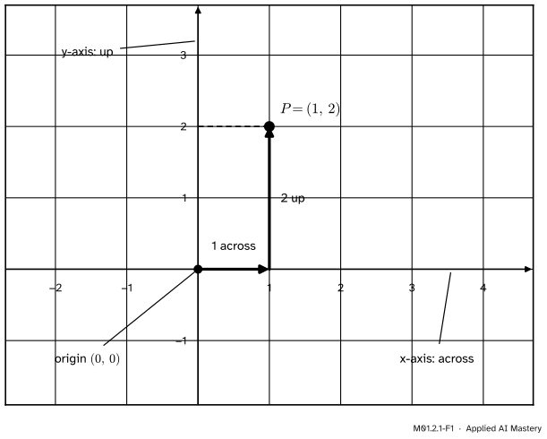
Now every point of the page has an address made of two numbers. To reach the point \(P\) in the figure, start at the origin, walk 1 across, then walk 2 up. We write \({P = (1, 2)}\): the across number first, the up number second.
M01.2.1-F1
The point \({P = (1, 2)}\): start at the origin, go 1 across, then 2 up. The first number is read on the x-axis and the second on the y-axis.
That is the whole idea: a pair of numbers is a place, and a place is a pair of numbers. Draw the pairs of a table as dots and you have a scatter plot. Machine learning looks at a data table in the same way. Each row becomes a dot, and the page becomes a map of the data on which nearby dots are similar examples.
Build it up
Step 1. Coordinates. The two numbers that name a point are its coordinates. In \({P = (1, 2)}\), the number 1 is the x-coordinate and 2 is the y-coordinate. The pair is an ordered pair, because its order carries meaning. \((1, 2)\) means 1 across and 2 up. \((2, 1)\) means 2 across and 1 up, which is a different point. Swap the numbers and the point moves.
Step 2. Signs. A negative x-coordinate means walk left, and a negative y-coordinate means walk down. So \({(-3, 2)}\) is 3 to the left and 2 up. A zero means do not move that way: \((0, 5)\) sits on the y-axis and \((4, 0)\) sits on the x-axis.
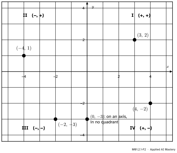
Step 3. Quadrants. The two axes cut the plane into four regions called quadrants. They are numbered I to IV, going anticlockwise from the top right. The two signs alone tell you which quadrant a point is in.
M01.2.1-F2
The signs of the two coordinates name the quadrant. A point with a zero coordinate lies on an axis and belongs to no quadrant.
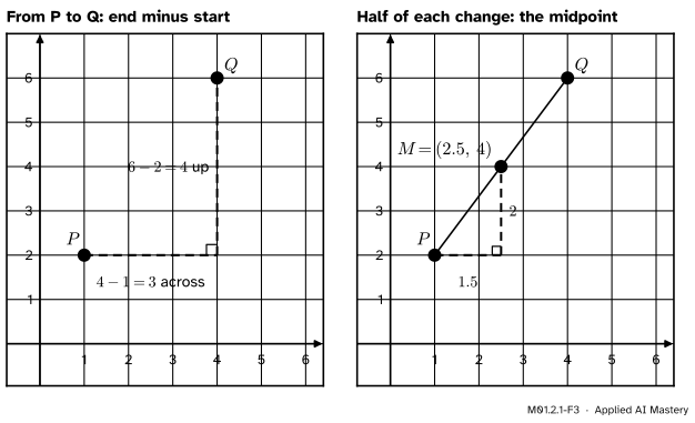
Step 4. From one point to another. Take \({P = (1, 2)}\) and \({Q = (4, 6)}\). To walk from \(P\) to \(Q\) you go some way across and some way up. Each amount is a subtraction, end minus start:
that is, 3 to the left and 4 down. The horizontal change is also called the run and the vertical change the rise. Lesson M01.3.2 uses those names for the slope of a line.
Step 5. Halfway. From \(P\), walk half of each change: 1.5 across and 2 up. You land on
\[
(1 + 1.5,\; 2 + 2) = (2.5,\; 4),
\]
the point halfway between \(P\) and \(Q\). It is called the midpoint. Look at its two numbers: 2.5 is the average of 1 and 4, and 4 is the average of 2 and 6. The midpoint is the average of the two points, one coordinate at a time.
M01.2.1-F3
Left: the walk from \(P\) to \(Q\) is 3 across and 4 up, each found by subtracting. Right: half of each change, walked from \(P\), lands on the midpoint \({M = (2.5, 4)}\).
The formal statement
NoteDefinition: the coordinate plane
The coordinate plane is a flat plane with two number lines at right angles: the horizontal x-axis and the vertical y-axis, crossing at the origin\((0, 0)\). Each point \(P\) is named by an ordered pair\({P = (p_1, p_2)}\) of its x-coordinate \(p_1\) and its y-coordinate \(p_2\). Two pairs name the same point exactly when their first coordinates agree and their second coordinates agree.
The small numbers are labels, as in lesson M01.1.4: \(p_1\) is the first coordinate of \(P\) and \(p_2\) is its second. A second point is written \({Q = (q_1, q_2)}\). Three results follow.
The second line multiplies out the bracket (the distributive law of M01.1.2). The third line collects the two terms in \(p_1\): one whole \(p_1\) take away half of it leaves half of it. The same four lines with the second coordinates give \(m_2\), so
The bar means “the mean of”, as in M01.1.4. With \({n = 2}\) this is the midpoint formula again, so the midpoint is the mean point of two points.
Frontier note: centring a data set on its mean point
Many methods start by sliding a whole data set so that its mean point sits at the origin: subtract \(\bar{x}\) from every x-coordinate and \(\bar{y}\) from every y-coordinate. This is called centring. The course’s four points, whose mean point is \((2.5, 4)\) (worked below), become \({(-1.5, -2)}\), \({(-0.5, -1)}\), \((0.5, 1)\) and \((1.5, 2)\), and their new mean point is \((0, 0)\). Standardising features (ML01.3.3) and principal component analysis (M03.6) both begin with this step.
Worked example
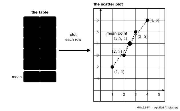
The course’s four data points, from table to picture. The table has one row per example: an input \(x\) and a target \(y\).
M01.2.1-F4
Each row of the table becomes one dot. The mean point \((2.5, 4)\) is also the midpoint of the outer pair and of the inner pair.
Plot the rows. Each row \((x, y)\) is a point: go \(x\) across and \(y\) up. Both coordinates of every point are positive, so all four dots lie in quadrant I.
Find the mean point. Add each column and divide by the number of rows:
Compare it with a midpoint. The first point is \({P = (1, 2)}\) and the last is \({Q = (4, 6)}\). Their midpoint, from Step 5, is also \((2.5, 4)\). That is not luck. The two inner points have the midpoint
as well. The data come in two pairs, each balanced around \((2.5, 4)\), so the average of all four is that same point.
Code
First from scratch. A point is a tuple, two numbers in round brackets, and Python counts its positions from 0: P[0] is the x-coordinate and P[1] is the y-coordinate.
P = (1, 2) # the point P: across 1, up 2Q = (4, 6) # the point Qacross = Q[0] - P[0] # horizontal change: end minus startup = Q[1] - P[1] # vertical change: end minus startprint("from P to Q:", across, "across and", up, "up")midpoint = [] # an empty list, filled one coordinate at a timefor k inrange(2): # k is 0, then 1 midpoint.append((P[k] + Q[k]) /2) # the average of the two coordinatesprint("midpoint:", midpoint)
from P to Q: 3 across and 4 up
midpoint: [2.5, 4.0]
The mean point of the four data points takes one loop that walks the two lists together, as P01.6.2 does with zip.
xs = [1, 2, 3, 4] # the x-coordinates of the four pointsys = [2, 3, 5, 6] # their y-coordinates, in the same ordertotal_x =0total_y =0for x, y inzip(xs, ys): # one point at a time total_x = total_x + x total_y = total_y + ymean_point = (total_x /len(xs), total_y /len(ys))print("mean point:", mean_point)
mean point: (2.5, 4.0)
Now the same with NumPy, as a preview of P02. One array holds the whole table, with a row per point and a column per coordinate.
import numpy as nppoints = np.array([[1, 2], [2, 3], [3, 5], [4, 6]]) # one row per pointprint(points.shape) # (rows, columns)print(points.mean(axis=0)) # axis=0 averages down each column
(4, 2)
[2.5 4. ]
The shape (4, 2) says 4 points with 2 coordinates each, and the column means are the mean point. Drawing the scatter plot takes two lines of Matplotlib, which P02.8 teaches. They are shown here, not run; figure M01.2.1-F4 was drawn by a longer script of the same kind.
import matplotlib.pyplot as pltplt.scatter(xs, ys) # one dot for each (x, y) pair
Every scatter plot rests on this lesson, and so does every feature space in machine learning: a table with two numeric columns is a set of points in the plane.
Explore
This module’s interactive, the point and arrow explorer, lives in lesson M01.2.4, where it also shows arrows. You can use it now: drag the two points, or move their sliders, and watch the horizontal change, the vertical change and the midpoint update.
Pitfalls
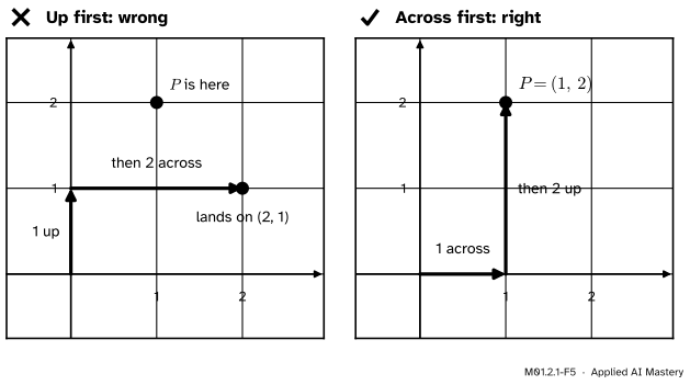
M01.2.1-F5
Wrong beside right. Reading the pair as “up, then across” lands on \((2, 1)\), a different point. The first number is always the across number.
“\((1, 2)\) and \((2, 1)\) contain the same numbers, so they are the same point.”
The order is part of the address. The first number is how far across and the second how far up, so \((1, 2)\) and \((2, 1)\) sit in different places. Swapping the two columns of a data table would move every one of its dots.
“A change is a length, so it can never be negative.”
A change keeps its sign, because it says which way to go. From \({Q = (4, 6)}\) to \({P = (1, 2)}\) the changes are \({-3}\) across and \({-4}\) up. A distance is never negative, and lesson M01.2.3 builds one from these changes, but the changes themselves can be.
“Half the change is the midpoint.”
Half of each change, 1.5 across and 2 up, tells you how far to walk from\(P\). The midpoint is where you land: \((2.5, 4)\). A quick check catches the slip. Each coordinate of the midpoint is equally far from the matching coordinates of the two points: 2.5 is 1.5 away from both 1 and 4, and 4 is 2 away from both 2 and 6. The wrong answer \((1.5, 2)\) fails at once, because 2 is no distance from 2 but 4 away from 6.
“P[1] is the first coordinate.”
In maths the first coordinate of \(P\) is \(p_1\). In Python it is P[0], because Python counts from 0 (M01.1.4). P[1] is the second coordinate, the y-coordinate.
Check yourself
Recall
1. In the ordered pair \((x, y)\), which number tells you how far across and which tells you how far up?
Show answer
The first number, \(x\), is how far across. The second number, \(y\), is how far up.
2. Which quadrant holds the point \({(-3, 2)}\), and why?
Show answer
Quadrant II. Its x-coordinate is negative (left of the y-axis) and its y-coordinate is positive (above the x-axis), the sign pattern \({(-, +)}\).
3. What are the horizontal and the vertical change from \((4, 6)\) to \((1, 2)\)?
The point whose x-coordinate is the mean of all the x-coordinates and whose y-coordinate is the mean of all the y-coordinates.
Exercises
1.★ Say where each point lies: in which quadrant, or on which axis. \({A = (3, -1)}\), \({B = (-2, -4)}\), \({C = (0, 5)}\), \({D = (-0.5, 2)}\).
Show solution
\(A\) has signs \({(+, -)}\), so it is in quadrant IV. \(B\) has \({(-, -)}\), so it is in quadrant III. \(C\) has x-coordinate 0, so it lies on the y-axis and in no quadrant. \(D\) has \({(-, +)}\), so it is in quadrant II.
2.★★ Let \({P = (-1, 3)}\) and \({Q = (5, -1)}\). Find the horizontal and the vertical change from \(P\) to \(Q\), and the midpoint \(M\). Check \(M\) by walking half of each change from \(P\).
Check: half of each change is 3 across and \({-2}\) up. From \(P\) that lands on
\[
(-1 + 3,\; 3 - 2) = (2,\; 1),
\]
the same point.
3.★★★ The point \({M = (2.5, 4)}\) is the midpoint of \({P = (1, 2)}\) and a point \(Q\) that has been lost. Find \(Q\). Then find a rule that gives \(Q\) from any \(P\) and \(M\).
The same steps with the second coordinates give \({q_2 = 2m_2 - p_2}\). In words: double the midpoint and take away the known end. Check both with the numbers:
A point is two numbers: how far across, then how far up.
M01.2.1-F1
Across first, then up.
A point:\({P = (p_1, p_2)}\), the x-coordinate first. The signs give the quadrant.
Change from \(P\) to \(Q\):\({q_1 - p_1}\) across and \({q_2 - p_2}\) up, signs kept.
Midpoint: the average of the two points, one coordinate at a time.
Mean point:\((\bar{x}, \bar{y})\), the average of all the points.
Sources and next steps
Sources. Each was opened and checked against this lesson on 12 November 2026.
OpenStax, Prealgebra 2e, Section 11.1, “Use the Rectangular Coordinate System”. It defines the axes, the origin and the ordered pair, notes that the order of the coordinates matters with \((1, 3)\) and \((3, 1)\), numbers the quadrants anticlockwise from the upper right and tabulates their signs.
OpenStax, Algebra and Trigonometry 2e, Section 2.1, “The Rectangular Coordinate Systems and Graphs”. It gives the midpoint formula under “Using the Midpoint Formula”.
Marc Peter Deisenroth, A. Aldo Faisal and Cheng Soon Ong, Mathematics for Machine Learning, Section 8.1.1, “Data as Vectors”. Each row of a data table is one example and each column one feature, so each example is a list of numbers, one per feature.
NumPy, numpy.mean. The axis argument; its example np.mean(a, axis=0) for the rows [1, 2] and [3, 4] gives [2., 3.], the mean of each column.